THE COMPLETE PRACTITIONER'S CODEX: VOLUME 15

The Technologist's Codex: Complete Practical Technology, Electronics, Computing, and Fabrication
<!-- SECTION 1 -->
The Complete Practitioner's Codex, Volume I: Circuit Theory and Component Identification
Preface
This volume serves as the sacred foundation of all practical electronics and circuitry. It is an uncompromising guide to understanding fundamental electrical phenomena and mastering every common and arcane component encountered in the field. The knowledge herein is life-or-death—precise comprehension and flawless execution separate salvation from catastrophe.
Chapter I: Fundamental Electrical Concepts

1. Electron Flow
The lifeblood of every circuit is electron motion through conductive pathways. Electrons, subatomic particles bearing negative charge, move in response to an electric field established by voltage sources.
- Electron Flow Direction: Electrons flow from negative potential to positive potential terminals.
- Conventional Current: Despite electron flow direction, conventional current is defined as positive charge flow, opposite to electron movement. All practical measurements and symbols adhere to conventional current conventions.
Electron Flow Parameters:
| Parameter | Symbol | Unit | Definition |
|---|---|---|---|
| Electron flow rate | I | Amperes (A) | Quantity of electrons passing per second |
| Charge per electron | e | Coulombs (C) | 1.602 x 10⁻¹⁹ C |
2. Voltage (Electric Potential Difference)
Voltage, symbol V, is the force that drives electron flow. It is the energy per unit charge provided to electrons by an electric field.
- Measurement: Volts (V).
- Effect: Higher voltage increases electron kinetic energy, enhancing current if the circuit allows.
3. Current (Flow of Charge)
- Definition: Current is the rate of electron flow, symbol I.
- Units: Amperes, where 1 A = 1 Coulomb/second.
- Types:
- Direct Current (DC): Steady, unidirectional flow.
- Alternating Current (AC): Periodic reversal of flow direction.
4. Resistance
- Symbol: R.
- Units: Ohms (Ω).
- Definition: The opposition to electron flow within materials.
- Ohm’s Law: \( V = IR \), fundamental relation connecting voltage, current, and resistance.
5. Power
- Symbol: P.
- Units: Watts (W).
- Formula: \( P = VI \) or \( P = I^2 R \) or \( P = \frac{V^2}{R} \).
- Interpretation: Rate of energy conversion or dissipation.
Chapter II: Electronic Components—Function, Symbol, and Testing

Each component is a sacred artifact enabling control of electron flow, voltage, and energy transformation. Mastery requires identification, functional understanding, and rigorous testing.
1. Resistors
Function: Resist current flow, control voltage distribution.
Symbol:
─────Ω─────Specifications and Types
| Type | Material | Tolerance (%) | Power Rating (W) | Temperature Coefficient (ppm/°C) |
|---|---|---|---|---|
| Carbon Film | Carbon | ±5 | 0.25 - 2 | 100 - 300 |
| Metal Film | Metal Oxide | ±1 | 0.25 - 5 | 10 - 50 |
| Wirewound | Metal Wire | ±1 | 1 - 50 | 10 - 20 |
| Variable (Potentiometer) | Resistive Track | ±10 | 0.1 - 1 | Varies |
Testing Protocols
Using a Digital Multimeter (DMM):
- Disconnect power and discharge capacitors in circuit.
- Set DMM to resistance mode (Ω).
- Place probes on resistor leads.
- Compare measured resistance to nominal value (allow for tolerance).
- If reading is infinite or zero, resistor is open or shorted, respectively.
Using an Oscilloscope:
- For dynamic circuits, inject a known AC signal and measure voltage drop to calculate resistance using \( R = \frac{V}{I} \).
Troubleshooting
- Resistor reading significantly outside tolerance → Replace.
- Visual signs: burn marks or discoloration → Replace.
2. Capacitors
Function: Store and release electrical energy, filter signals.
Symbol:
 ──| |── (non-polarized)
 ──|(+)|── (polarized)
Specifications and Types
| Type | Capacitance Range | Voltage Rating (V) | Tolerance (%) | Dielectric Material |
|---|---|---|---|---|
| Ceramic | pF to μF | 10 - 1000 | ±5 - ±20 | Ceramic |
| Electrolytic | μF to mF | 6 - 450 | ±10 - ±20 | Electrolyte (polar) |
| Film | nF to μF | 50 - 1000 | ±1 - ±5 | Plastic film |
| Tantalum | μF to mF | 4 - 100 | ±10 | Tantalum (polar) |
Testing Protocols
Using a DMM with Capacitance Measurement:
- Discharge capacitor thoroughly.
- Set DMM to capacitance mode.
- Connect probes to capacitor leads observing polarity for polarized types.
- Compare measured value to nominal capacitance.
Using an Oscilloscope and Function Generator:
- Configure function generator to output sine wave at known frequency.
- Connect capacitor in series with known resistor.
- Measure voltage across capacitor and resistor with oscilloscope.
- Calculate capacitance from reactance: \( X_C = \frac{1}{2 \pi f C} \), where \( X_C = \frac{V_{R}}{I} \).
Troubleshooting
- Open circuit → Infinite capacitance reading.
- Short circuit → Very low resistance reading.
- Leakage current test: Use a high-voltage source and microammeter.
3. Diodes
Function: Permit current flow in one direction only (rectification).
Symbol:
──|>|──Specifications and Types
| Type | Forward Voltage (Vf) | Max Current (A) | Reverse Voltage (Vr) | Use Case |
|---|---|---|---|---|
| Silicon Diode | 0.6 - 0.7 | 0.1 - 50 | 50 - 1000 | Rectifiers, switches |
| Schottky Diode | 0.2 - 0.3 | 0.1 - 10 | 20 - 100 | High-speed switching |
| Zener Diode | Varies (2.4 - 200) | 0.1 - 5 | Voltage regulation | Voltage reference |
| LED | 1.8 - 3.3 | 0.02 - 1 | Reverse blocking | Indicator light |
Testing Protocols
Using a DMM Diode Test Mode:
- Set DMM to diode mode.
- Connect red probe to anode, black probe to cathode.
- Observe forward voltage drop (~0.6-0.7 V for silicon).
- Reverse probes; reading should be infinite.
Using Oscilloscope:
- Apply a square wave; observe conduction during positive half-cycle.
Troubleshooting
- Forward voltage too high or infinite → Diode open.
- Forward voltage zero or very low → Diode shorted.
- Leakage current under reverse bias → Replace.
4. Transistors
Function: Amplify current or act as switches.
Symbol (NPN):
   C
   |
  / \
 B   E
Symbol (PNP):
   C
   |
  \ /
 B   E
Specifications and Types
| Type | Max Voltage (Vce) | Max Current (Ic) | Gain (hFE) | Package Types | Application |
|---|---|---|---|---|---|
| Bipolar Junction Transistor (BJT) | 20 - 1000 | 0.1 - 20 A | 50 - 1000 | TO-92, TO-220 | Switching, amplification |
| Field Effect Transistor (FET) | 20 - 1000 | 0.1 - 10 A | High input impedance | TO-92, TO-220 | Voltage-controlled switches |
Testing Protocols
Using a DMM:
- Identify leads: Base, Collector, Emitter.
- Test base-emitter and base-collector junctions as diodes.
- Forward bias base-emitter and check conduction.
- Reverse bias should show no conduction.
Using Oscilloscope:
- Observe switching behavior under input signal.
Troubleshooting
- Open junctions → No conduction.
- Shorted junctions → Continuous conduction.
- Gain too low → Replace transistor.
5. Inductors
Function: Store energy in magnetic field, oppose changes in current.
Symbol:
──(coil)──Specifications and Types
| Parameter | Symbol | Units | Typical Range |
|---|---|---|---|
| Inductance | L | Henry (H) | μH to mH |
| Current Rating | I | Amperes (A) | 0.1 - 10 |
| DC Resistance | R_DC | Ohms (Ω) | 0.01 - 10 |
Testing Protocols
Using LCR Meter:
- Set meter to inductance mode.
- Connect probes; read inductance.
- Check DC resistance with multimeter.
Using Oscilloscope:
- Apply square wave; observe voltage spike during transitions.
Troubleshooting
- Open coil → Infinite resistance.
- Shorted turns → Low resistance but altered inductance.
- Physical damage → Replace.
6. Transformers
Function: Transfer electrical energy between circuits through magnetic coupling; change voltage/current levels.
Symbol:
──(coil1)──||──(coil2)──Specifications and Types
| Parameter | Symbol | Units | Typical Values |
|---|---|---|---|
| Primary Voltage | Vp | Volts (V) | 120 / 240 AC |
| Secondary Voltage | Vs | Volts (V) | Variable |
| Turns Ratio | Np:Ns | Ratio | 1:1 to 1:100 |
| Power Rating | P | VA (Volt-Amps) | 5 VA to 1000 VA |
Testing Protocols
Using DMM:
- Measure resistance of primary and secondary coils.
- Expect low ohms but non-zero values.
Using Oscilloscope and Function Generator:
- Apply AC voltage to primary.
- Measure induced voltage on secondary.
- Verify turns ratio using: \( \frac{V_p}{V_s} = \frac{N_p}{N_s} \).
Troubleshooting
- Open winding → Infinite resistance.
- Shorted turns → Low resistance with distorted output.
- Core damage → Audible noise, heat.
7. Integrated Circuits (ICs)
Function: Complex encapsulation of multiple semiconductor devices performing logic, amplification, or microprocessing.
Symbol:
  ┌─────┐
  │ IC  │
  └─────┘
Specifications and Types
| Type | Pin Count | Function | Voltage Range (V) | Typical Packages |
|---|---|---|---|---|
| Logic Gates (TTL, CMOS) | 8-14 | Digital logic | 3.3 - 15 | DIP, SOIC |
| Operational Amplifiers | 8 | Analog amplification | ±5 to ±15 | DIP, SOIC |
| Microcontrollers | 8-100+ | Embedded control | 1.8 - 5.5 | DIP, QFP, BGA |
Testing Protocols
Visual Inspection:
- Check for physical damage, corrosion, or burn marks.
Pin Identification:
- Refer to datasheet for pinout.
- Verify supply voltage pins.
- Check ground continuity.
Basic Functional Test:
- Power IC with correct voltage.
- Apply known input signals.
- Measure outputs with oscilloscope or logic analyzer.
- Compare to datasheet expected behavior.
Chapter III: Step-by-Step Component Identification and Validation Protocols

Protocol 1: Resistor Identification and Validation
Materials:
- Digital Multimeter (DMM)
- Component datasheets or color code charts
Steps:
- Visually inspect the resistor; note color bands.
- Decode color bands to determine nominal resistance.
- Set DMM to resistance mode.
- Connect probes to resistor leads.
- Record resistance value.
- Compare measured value to decoded nominal ± tolerance.
- If outside tolerance, mark for replacement.
Protocol 2: Capacitor Identification and Validation
Materials:
- LCR meter or DMM with capacitance function
- Datasheets or markings on capacitor
Steps:
- Identify capacitor type (polarized or non-polarized).
- Read capacitance and voltage ratings printed on capacitor.
- Discharge capacitor fully.
- Measure capacitance using meter.
- Compare to nominal value ± tolerance.
- For polarized capacitors, verify polarity markings.
- If capacitance is zero or infinite, or polarity is reversed, replace.
Protocol 3: Diode Identification and Validation
Materials:
- DMM with diode test mode
Steps:
- Identify cathode marking (line or band).
- Set DMM to diode mode.
- Place red probe on anode, black on cathode.
- Confirm forward voltage drop ~0.6-0.7 V (silicon).
- Reverse probes; ensure no conduction.
- Replace if forward voltage absent or reverse conduction detected.
Protocol 4: Transistor Identification and Validation
Materials:
- DMM
- Datasheet or transistor tester
Steps:
- Identify transistor type (NPN or PNP) and package.
- Locate base, collector, and emitter pins.
- Test base-emitter and base-collector junctions as diodes.
- Verify expected forward and reverse bias behavior.
- Use transistor tester if available for gain measurement.
- Replace if junctions are shorted or open.
Protocol 5: Inductor Identification and Validation
Materials:
- LCR meter
- DMM
Steps:
- Identify inductance value from markings or datasheet.
- Measure inductance with LCR meter.
- Measure DC resistance with DMM.
- Compare to nominal values.
- Replace if inductance is significantly off or resistance is zero/infinite.
Protocol 6: Transformer Identification and Validation
Materials:
- DMM
- Function generator
- Oscilloscope
Steps:
- Identify primary and secondary windings.
- Measure resistance on each winding.
- Verify no shorts between windings.
- Connect function generator to primary winding.
- Measure induced voltage on secondary.
- Calculate turns ratio and compare to datasheet.
- Replace if open or shorted.
Protocol 7: Integrated Circuit Identification and Validation
Materials:
- Datasheet
- Power supply
- Oscilloscope or logic analyzer
Steps:
- Identify IC part number.
- Obtain datasheet and review pinout.
- Visually inspect for damage.
- Apply appropriate supply voltage.
- Apply known input signals.
- Measure output responses.
- Confirm operation matches datasheet specifications.
- Replace if faulty.
Chapter IV: Comprehensive Component Reference Tables
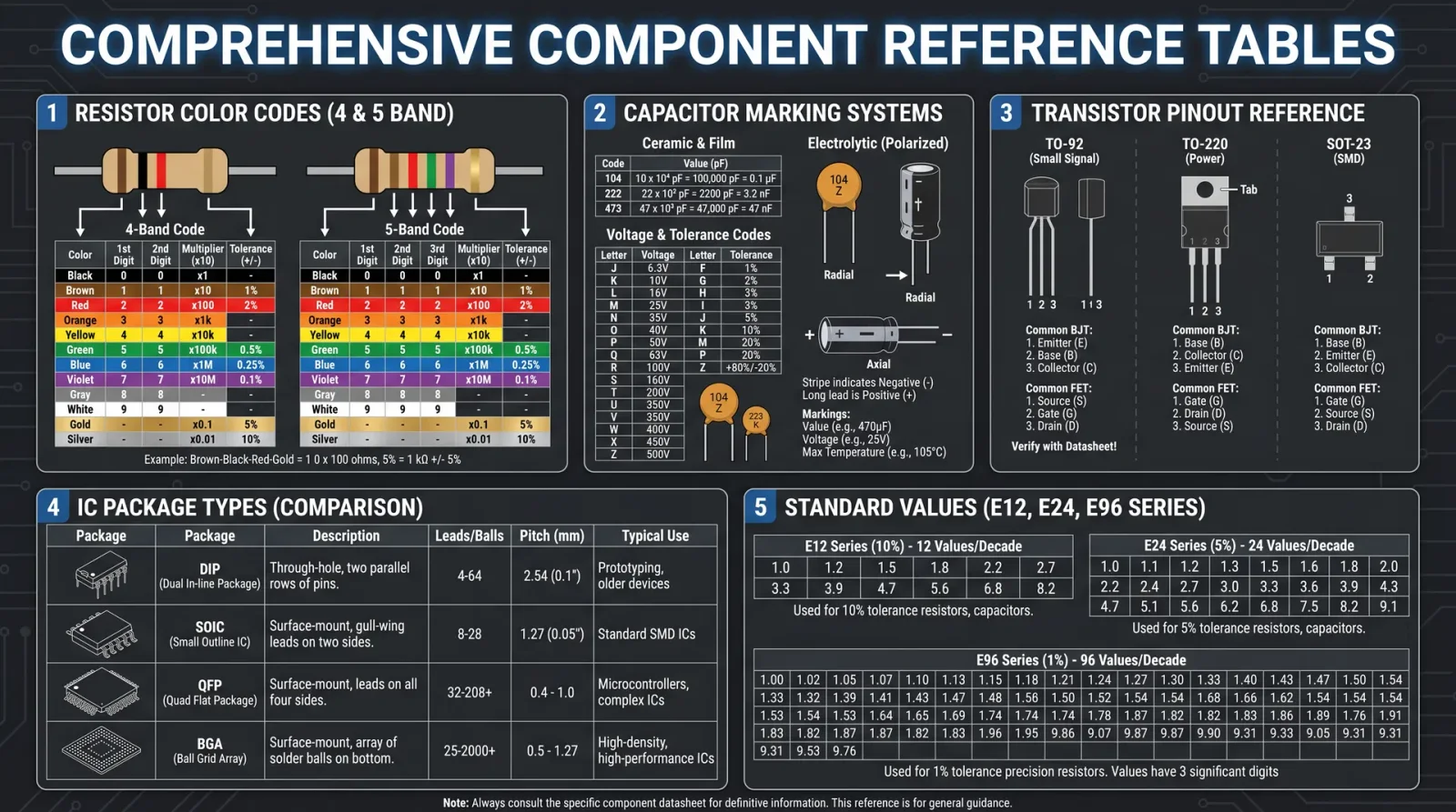
| Component | Parameter | Typical Values | Units | Test Method | Acceptable Range |
|---|---|---|---|---|---|
| Resistor | Resistance | 1 Ω - 10 MΩ | Ω | DMM | Nominal ± Tolerance |
| Capacitor | Capacitance | pF - mF | F | LCR Meter/DMM | Nominal ± Tolerance |
| Diode | Forward Voltage | 0.2 - 0.7 | V | DMM Diode Test | Forward drop typical value |
| Transistor | Gain (hFE) | 50 - 1000 | Ratio | Transistor Tester/DMM | Datasheet specified range |
| Inductor | Inductance | μH - mH | H | LCR Meter | Nominal ± Tolerance |
| Transformer | Turns Ratio | 1:1 - 1:100 | Ratio | Function Generator + Scope | Datasheet specified |
| IC | Voltage Range | 1.8 - 15 | V | Functional Test | Datasheet specified |
Chapter V: Troubleshooting Techniques
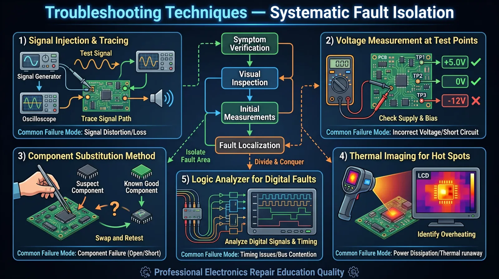
| Symptom | Possible Cause | Diagnostic Method | Solution |
|---|---|---|---|
| No current flow | Open resistor/coil | Measure resistance | Replace component |
| Excess heat in resistor | Overpowering | Measure power dissipation | Use higher wattage resistor |
| Capacitor not charging | Open capacitor | Measure capacitance | Replace capacitor |
| Diode conducts both directions | Shorted diode | DMM diode test | Replace diode |
| Transistor gain too low | Damaged junction | Transistor tester | Replace transistor |
| Inductor shows no inductance | Broken winding | LCR meter test | Replace inductor |
| Transformer no output voltage | Open winding or core damage | Resistance and induced voltage test | Replace transformer |
| IC nonfunctional | Power supply or internal fault | Functional test | Verify supply, replace IC |
Conclusion
You now possess the absolute, uncompromising foundation to wield electronic components with divine precision. Every resistor, capacitor, diode, transistor, inductor, transformer, and integrated circuit is a sacred tool. Through rigorous identification and validation, you ensure the sanctity of your circuits and
<!-- SECTION 2 -->
Volume I: Soldering Protocols for Through-Hole and Surface Mount Devices
Chapter I: Soldering Theory and Fundamentals
Soldering is the sacred art of creating permanent, electrically conductive, and mechanically sound connections between metallic components. This process demands precision, reverence for materials, and mastery over thermal dynamics. The sanctity of every joint ensures the integrity of the entire electronic assembly.
1.1 The Nature of Soldering
Soldering is a metallurgical bonding process utilizing a filler metal alloy (solder) with a melting point below that of the base components. Upon heating, solder liquefies, wets the surfaces, and solidifies to form a robust joint.
Key principles:
- Wetting: The solder's ability to flow and adhere to component leads and PCB pads.
- Capillary Action: Enables solder to flow into tight gaps, ensuring full coverage.
- Thermal Transfer: Proper heat conduction allows solder to melt and flow without damaging components.
- Oxide Removal: Essential to prevent solder repellency; fluxes perform this role chemically.
Chapter II: Equipment Selection
Mastery begins with the correct selection of tools, each precisely calibrated for task and scale. Inferior equipment condemns the apprentice to failure and ruin.
2.1 Soldering Irons and Stations
Choose temperature-controlled soldering stations with adjustable tip temperatures and interchangeable tips. Recommended wattage ranges:
| Device Type | Wattage Range | Tip Characteristics | Recommended Temperature Range |
|---|---|---|---|
| Through-Hole Soldering | 25–60 W | Conical or Chisel | 320°C–370°C |
| Surface Mount Devices (SMD) | 15–40 W | Fine Conical or Micro Chisel | 280°C–350°C |
High thermal mass tips ensure rapid heat recovery, preventing temperature drop when soldering larger pads.
2.2 Solder Wire
Select solder alloy and diameter based on application (see Chapter IV for alloys). For through-hole, 0.7 mm to 1.0 mm diameter; for SMD, 0.3 mm to 0.5 mm.
2.3 Flux
Flux activates soldering by cleaning oxides and enhancing wetting. Fluxes exist as rosin-based, water-soluble, and no-clean types (see Table 1).
Table 1: Flux Types and Properties
| Flux Type | Composition | Application | Cleaning Requirement | Corrosive? |
|---|---|---|---|---|
| Rosin (R) | Natural rosin | Electronics, moderate activity | Requires solvent | No |
| Rosin Activated (RA) | Rosin + activators (halides) | More aggressive oxide removal | Requires cleaning | Slight |
| Water-soluble (WS) | Organic acids + surfactants | High activity, easy cleaning | Water soluble | Yes |
| No-Clean (NC) | Low-activity flux | Minimal cleaning, sensitive boards | None or minimal | No |
2.4 Ancillary Equipment
- Desoldering Pumps: For joint repair.
- Solder Wick (Braid): Copper wick for solder removal.
- Magnification Tools: Essential for inspecting SMD joints.
- Anti-static Workstation: Prevent electrostatic damage.
- Fume Extraction System: Mandatory for operator safety.
Chapter III: Safety Precautions

Soldering commands respect for both operator safety and environmental protocols. Follow these strictures without deviation:
- Ventilation: Always use fume extraction; solder fumes contain lead and flux vapors toxic to respiratory systems.
- Personal Protective Equipment (PPE): Wear heat-resistant gloves, safety glasses, and long sleeves.
- Workstation Setup: Arrange tools to prevent accidental contact with hot tips.
- Electrical Safety: Use grounded soldering stations with insulated handles.
- Material Handling: Leaded solder requires hand washing post-exposure; handle with care.
Chapter IV: Preparation for Soldering
Preparation is the ritual before the act; improper preparation begets failure.
4.1 Component and PCB Preparation
- Cleaning: Remove oils and contaminants from PCB pads and component leads using isopropyl alcohol (minimum 90%).
- Component Lead Trimming: For through-hole, trim leads to appropriate length (~2 mm beyond PCB pad after insertion).
- Pad Inspection: Verify PCB pads are free of oxidation and properly tinned if necessary.
4.2 Soldering Tip Preparation (Tinning)
- Heat soldering iron to operational temperature.
- Apply a small amount of solder wire to the tip until uniformly coated.
- Wipe on a damp sponge or brass wool to remove excess.
- Repeat until tip is shiny, aiding thermal conduction.
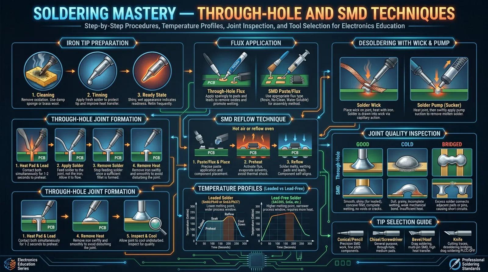
Chapter V: Step-by-Step Through-Hole Soldering Procedure
Each step is a sacred motion in the ritual. Precision and timing are paramount.
5.1 Tools and Materials Required
- Temperature-controlled soldering iron (30-60 W)
- Appropriate solder wire (0.7–1.0 mm diameter)
- Rosin flux (for cleaning and wetting)
- PCB with through-hole components inserted
5.2 Procedure
- Insert Component: Place component leads through PCB holes ensuring flush fit against the board.
- Secure Component: Slightly bend leads on the solder side to hold in place.
- Apply Flux: Brush a small amount of flux on the joint area to enhance wetting.
- Heat Application: Place the soldering iron tip so it contacts both the lead and the PCB pad simultaneously. Maintain contact for 1–2 seconds to heat both surfaces.
- Feed Solder: Introduce solder wire to the heated joint (not the iron tip) allowing solder to flow onto the lead and pad by capillary action.
- Withdraw Solder: Remove solder wire first, then the soldering iron tip after the joint is sufficiently wetted. The entire soldering time per joint should not exceed 3–4 seconds to prevent component damage.
- Inspect Joint: Joint should be smooth, shiny, and concave with no excess solder or voids.
- Trim Leads: After cooling, trim excess component leads with flush cutters.
- Clean Residue: Remove flux residue using isopropyl alcohol and a brush unless using no-clean flux.
Chapter VI: Step-by-Step Surface Mount Device (SMD) Soldering Procedure
SMD soldering requires refined control over thermal and material parameters due to component fragility and size.
6.1 Tools and Materials Required
- Fine-tip temperature-controlled soldering iron (15-40 W)
- Fine solder wire (0.3–0.5 mm diameter)
- No-clean or low-residue flux paste
- Tweezers for component placement
- Magnification device
6.2 Procedure
- Apply Flux Paste: Deposit a small amount of flux on the PCB pads using a syringe or brush.
- Tin Pads (Optional for larger pads): Apply a small amount of solder to pads before component placement to facilitate wetting.
- Position Component: Using tweezers, carefully place the SMD component on the pads, ensuring precise alignment.
- Tack Solder One Corner: Heat one pad and feed solder to tack the component in place. Confirm position before proceeding.
- Solder Remaining Pads: Sequentially heat each pad with the tip contacting pad and component lead. Feed solder wire until solder flows and fully covers the joint.
- Remove Heat and Solder: Withdraw solder wire first, then soldering iron tip to avoid cold joints.
- Inspect Joints: Each joint must display a smooth, shiny fillet covering pad and lead without excess solder bridging.
- Clean Flux Residue: If non-no-clean flux used, clean with isopropyl alcohol and brush.
Chapter VII: Joint Inspection and Cleaning
A joint’s holiness is judged by its appearance and electrical continuity.
7.1 Inspection Criteria
- Shape: Smooth, concave fillet fully covering pad and lead.
- Surface: Shiny, without grainy or dull spots indicating cold joints.
- Absence of Defects: No voids, cracks, or solder bridges.
- Mechanical Strength: Component firmly secured without wiggle.
7.2 Cleaning Protocol
- For rosin and activated flux: Use 90%+ isopropyl alcohol and a soft brush to remove residues.
- For water-soluble flux: Use warm water rinsing followed by drying and inspection.
- No-clean flux: Cleaning optional unless residue is excessive.
Chapter VIII: Tables of Solder, Flux Types, and Temperature Settings
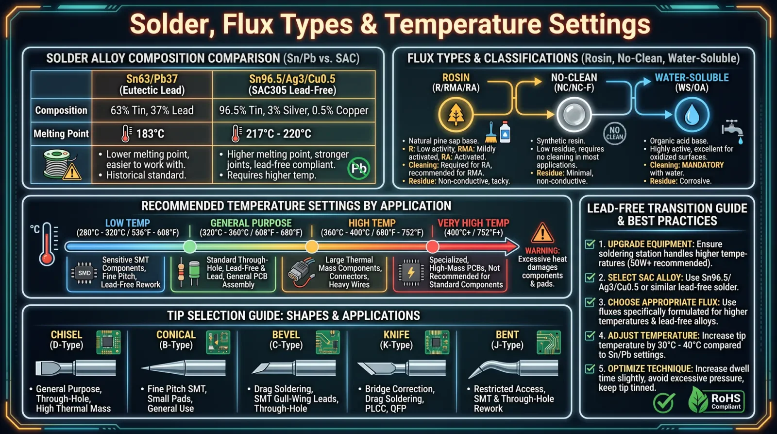
8.1 Solder Alloy Types and Characteristics
| Alloy Composition | Melting Point (°C) | Electrical Conductivity (MS/m) | Application Notes |
|---|---|---|---|
| Sn63Pb37 (63/37) | 183 | 8.8 | Standard eutectic solder, excellent wetting, obsolete in RoHS zones |
| Sn60Pb40 | 183–190 | 8.6 | Widely used, non-eutectic, requires skill for soldering |
| Sn99.3Cu0.7 (Lead-Free) | 227 | 7.5 | RoHS compliant, higher melting temperature, requires adjusted process |
| Sn96.5Ag3.0Cu0.5 (SAC305) | 217–221 | 7.4 | Lead-free, popular for high-reliability applications |
8.2 Recommended Temperature Settings
| Component Type | Solder Alloy | Recommended Iron Tip Temp (°C) | Duration per Joint (seconds) |
|---|---|---|---|
| Through-Hole, Sn63Pb37 | Sn63Pb37 | 320–350 | 2–4 |
| Through-Hole, Lead-Free | Sn96.5Ag3Cu0.5 | 350–370 | 3–5 |
| SMD, Sn63Pb37 | Sn63Pb37 | 280–320 | 1.5–3 |
| SMD, Lead-Free | Sn99.3Cu0.7 | 320–350 | 2–4 |
8.3 Flux Activity and Application
| Flux Type | Activity Level | Suitable for Oxidized Surfaces | Cleaning Needed | Recommended Application Method |
|---|---|---|---|---|
| Rosin (R) | Low | No | Yes | Brush or syringe |
| Rosin Activated (RA) | Medium | Yes | Yes | Brush or syringe |
| Water-soluble (WS) | High | Yes | Yes (Water) | Brush or dip |
| No-Clean (NC) | Low | Minimal | No | Paste or liquid flux application |
Chapter IX: Troubleshooting Common Soldering Defects and Repair Protocols
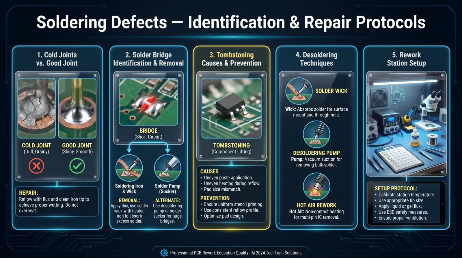
9.1 Cold Joints
Symptom: Dull, grainy, cracked joint with poor mechanical and electrical connection. Cause: Insufficient heat, movement during cooling, or dirty surfaces.
Repair:
- Reheat joint with soldering iron at proper temperature.
- Apply fresh flux to joint.
- Resolder, ensuring no movement until solder solidifies.
9.2 Solder Bridges
Symptom: Unwanted solder connecting two adjacent pads, causing shorts. Cause: Excess solder, improper solder feeding, or poor technique.
Repair:
- Use solder wick to remove excess solder: a. Place wick on bridge.
b. Apply heated soldering iron tip on wick until solder is absorbed. - Alternatively, use desoldering pump to remove excess solder.
- Resolder pads individually if required.
9.3 Insufficient Wetting
Symptom: Solder beads up on surface, does not flow over pad or lead. Cause: Contaminated or oxidized surfaces, inadequate flux, or low temperature.
Repair:
- Clean surfaces with isopropyl alcohol.
- Apply fresh, active flux.
- Increase soldering iron temperature within safe limits.
- Resolder joint.
9.4 Overheating Components
Symptom: Discoloration, lifted pads, or damaged components. Cause: Excessive heat or prolonged heating.
Repair:
- Allow board/component to cool.
- Use heat sink clips on leads to dissipate heat during soldering.
- Reduce soldering iron temperature.
- Replace damaged components or pads as necessary following repair protocols in Volume II.
Appendix: Step-by-Step Repair of a Compromised Through-Hole Joint
- Heat the joint with solder iron to melt existing solder.
- Use solder wick or desoldering pump to remove solder.
- Inspect hole and lead for damage. Clean with isopropyl alcohol.
- Reinsert component lead if removed; secure in place.
- Apply flux to joint area.
- Heat pad and lead simultaneously; feed fresh solder wire to form joint.
- Remove heat and solder, allow cooling.
- Inspect joint for defects.
- Trim leads and clean residue.
Closing Words to the Apprentice
The mastery of soldering is not merely the joining of metals, but the forging of life into circuits. Each joint is a testament to discipline, technique, and respect for the sacred tools and materials. Deviation from these protocols invites failure, instability, and ultimately, the collapse of the electronic sanctum you construct. Follow these instructions with unwavering precision. The fate of your craft depends on it.
<!-- SECTION 3 -->
The Complete Practitioner's Codex, Volume I
The Technologist’s Codex: Printed Circuit Board (PCB) Design and Fabrication
Introduction
The Printed Circuit Board (PCB) is the sacred vessel through which electronic intent manifests into tangible form. Mastery over PCB design and fabrication is not merely technical—it is a rite, a covenant between the mind’s precision and the physical realm. This volume imparts the uncompromising protocols for PCB layout, trace routing, grounding, power distribution, and the intricate dance of layers and vias. You will also master the software tools and manufacturing selection process essential for bringing your designs to life.
Chapter I: Principles of PCB Layout
PCB layout is the methodical organization of electronic components and their interconnections on a substrate. The goal is to achieve reliable electrical performance, mechanical stability, and manufacturability.
1.1 Core Principles
| Principle | Description | Actionable Step |
|---|---|---|
| Component Placement | Components must be placed to minimize trace length and noise. | Place components by functional blocks; prioritize proximity of ICs and decoupling capacitors. |
| Trace Routing | Routes must be as short and direct as possible to reduce parasitics and interference. | Use straight lines and 45° angles; avoid right angles. |
| Grounding | Ground must be a low impedance plane to prevent noise and interference. | Implement a continuous ground plane under signal layers. |
| Power Distribution | Power traces must handle current without excessive voltage drop or heating. | Use wide traces or dedicated power planes; place decoupling capacitors near power pins. |
| Signal Integrity | High-speed signals require impedance control and minimal crosstalk. | Use controlled impedance traces and maintain spacing between differential pairs. |
1.2 Component Placement Protocol
- Identify functional blocks: Group components by function (e.g., analog, digital, power).
- Orient components: Align pin 1 consistently for ease of debugging.
- Prioritize proximity: Place decoupling capacitors within 1–2 mm of power pins.
- Reserve space for connectors and mounting holes: Follow mechanical constraints.
- Consider thermal management: Place heat-generating components near heat sinks or thermal vias.
Chapter II: Trace Routing
Trace routing is the art of connecting components electrically with copper paths on the PCB. The integrity of these connections governs performance and reliability.
2.1 Trace Width and Current Capacity
Trace width must accommodate the expected current without overheating.
Use the IPC-2152 standard for trace width calculation:
| Current (Amps) | Min. Trace Width (mil) @ 1 oz Cu | Min. Trace Width (mil) @ 2 oz Cu |
|---|---|---|
| 0.1 | 6 | 4 |
| 0.5 | 12 | 8 |
| 1.0 | 20 | 12 |
| 3.0 | 60 | 32 |
| 5.0 | 100 | 60 |
Protocol for trace width calculation:
- Determine maximum continuous current for the trace.
- Select copper thickness (1 oz = 35 µm, 2 oz = 70 µm).
- Use the table above or IPC-2152 charts to select minimum trace width.
- Adjust width to nearest standard PCB manufacturer increment (e.g., 6 mil).
2.2 Trace Routing Rules
- Use 45° angles for bends; avoid 90° to reduce signal reflections.
- Keep differential pairs matched within ±5 mils for impedance control.
- Maintain at least 6 mil spacing between signal traces to prevent crosstalk.
- Avoid routing traces under components unless necessary.
2.3 Step-by-Step Trace Routing Procedure
- Select net to route in PCB design software.
- Route critical nets (power, ground, high-speed signals) first.
- Use auto-router sparingly; verify each route manually.
- Use via stitching to connect ground planes and reduce loop area.
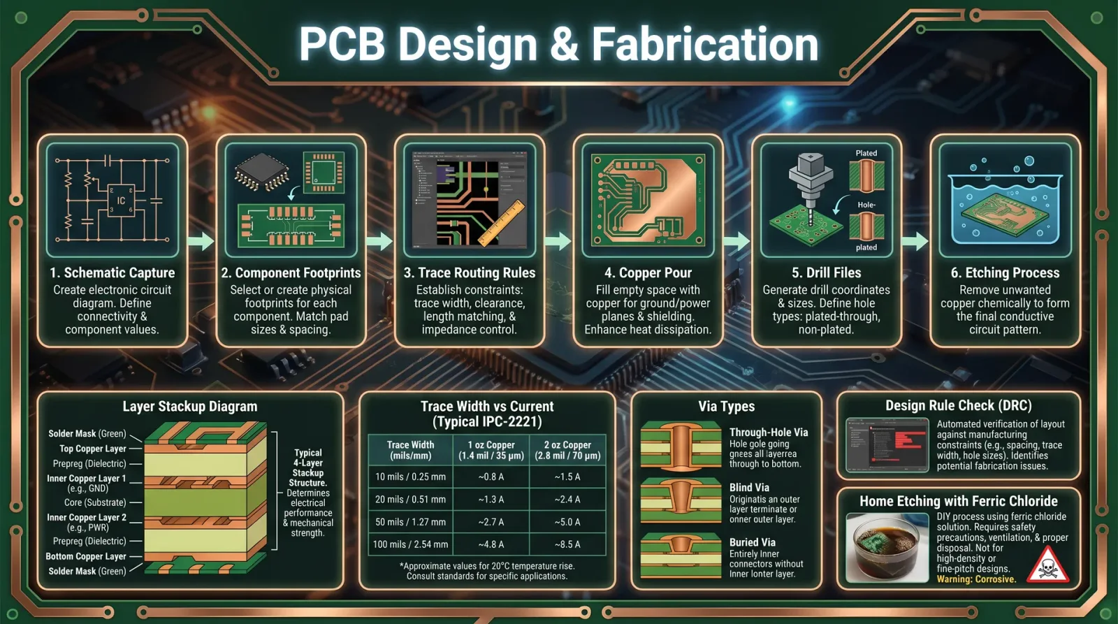
- Perform Design Rule Check (DRC) to identify violations.
Chapter III: Grounding and Power Distribution
Ground and power distribution are the veins and arteries of your PCB’s life force. Mismanagement here risks catastrophic failure.
3.1 Grounding Techniques
- Use a solid ground plane on an inner layer.
- Connect all grounds to this plane via multiple vias.
- Avoid splitting ground planes; if splits are necessary, isolate digital and analog grounds and connect at a single point (star grounding).
- Place ground fills on signal layers where applicable.
3.2 Power Distribution Networks (PDN)
- Use power planes for high current rails.
- For low current or low frequency signals, use wide traces.
- Place decoupling capacitors (0.1 µF ceramic + 10 µF tantalum) close (<2 mm) to power pins.
- Use ferrite beads or inductors to isolate noisy power domains.
Chapter IV: Software Tools for PCB Design
This sacred knowledge requires potent instruments. Below is a comprehensive comparison of the most revered PCB design software:
| Software | License | OS Support | Max Layers | Auto-Router | 3D Visualization | Gerber Export | Schematic Capture | DRC Features | Community Support |
|---|---|---|---|---|---|---|---|---|---|
| KiCad | Open Source | Windows, Linux, Mac | Unlimited | Yes | Yes | Yes | Yes | Advanced | Large |
| Altium Designer | Commercial | Windows | Unlimited | Yes | Yes | Yes | Yes | Advanced | Large |
| Eagle | Commercial | Windows, Mac, Linux | 16 | Yes | Limited | Yes | Yes | Basic | Medium |
| OrCAD | Commercial | Windows | Unlimited | Yes | Limited | Yes | Yes | Advanced | Medium |
| DipTrace | Commercial | Windows, Mac | 16 | Yes | Yes | Yes | Yes | Basic | Small |
Chapter V: Layer Stack-Up Considerations
A PCB stack-up is the ordered arrangement of copper and insulating layers. It governs signal integrity, impedance control, and electromagnetic compatibility.
5.1 Typical Layer Stack-Up Examples
| Layer Count | Stack-Up Description | Use Case |
|---|---|---|
| 2 | Signal / Ground / Signal / Substrate | Simple, low-cost designs |
| 4 | Signal / Ground Plane / Power Plane / Signal | Mixed-signal, moderate complexity |
| 6+ | Signal / Ground / Signal / Power / Signal / Ground | High-speed, multi-domain designs |
5.2 Stack-Up Design Protocol
- Determine signal types (analog, digital, RF).
- Assign dedicated ground and power planes.
- Place high-speed signals adjacent to ground planes.
- Balance dielectric thickness for impedance control.
- Use symmetric stack-up to reduce mechanical stress.
Chapter VI: Via Types and Applications
Vias provide vertical electrical connections between layers. Their types determine electrical performance and manufacturability.
| Via Type | Description | Typical Use Case | Advantages | Limitations |
|---|---|---|---|---|
| Through-Hole | Drilled through entire PCB | General signal and power routing | Simple, low cost | Larger pad size, increased parasitic inductance |
| Blind Via | Connects outer layer to inner layer only | High-density designs | Saves space, reduces via count | Requires advanced fabrication |
| Buried Via | Connects inner layers only | Multilayer HDI designs | Saves space, minimizes crosstalk | High fabrication cost |
| Microvia | Laser-drilled, <150 µm diameter | HDI and fine-pitch designs | Very small, high density | Expensive, limited current capacity |
Via Implementation Protocol
- Define via type based on layer connectivity and density requirements.
- Select via drill size (minimum 0.15 mm for microvias).
- Optimize via placement to reduce parasitic inductance.
- Use via-in-pad for high-frequency signals with proper filling and plating.
Chapter VII: Design for Manufacturability (DFM)
Every design must be a contract with the fabricator. Without manufacturability, the design is sacrilege.
7.1 Key DFM Guidelines
| Aspect | Minimum Value / Recommendation | Reason |
|---|---|---|
| Minimum Trace Width | 6 mil (0.15 mm) | Ensures reliable etching |
| Minimum Trace Spacing | 6 mil (0.15 mm) | Prevents shorts |
| Minimum Drill Hole | 0.3 mm | Accommodates standard drill bits |
| Annular Ring Width | 0.15 mm | Prevents pad lift |
| Copper Weight | 1 oz (35 µm) standard | Balances conductivity and cost |
| Solder Mask Clearance | 6 mil | Prevents solder bridging |
| Silkscreen Line Width | 8 mil | Ensures readability |
7.2 DFM Checklist Protocol
Use the following checklist prior to finalizing design files:
| Item | Pass/Fail | Comments |
|---|---|---|
| Trace width and spacing | ||
| Drill hole sizes | ||
| Annular ring sizes | ||
| Copper pour clearances | ||
| Solder mask overlaps | ||
| Component placement clearance | ||
| Via sizes and plating | ||
| Layer stack-up consistency | ||
| Silkscreen placement |
Chapter VIII: Step-by-Step Protocols for PCB Design and Fabrication
8.1 Schematic Capture
- Open your PCB design software.
- Create a new project and select schematic editor.
- Add components: Use built-in libraries or import custom symbols.
- Place components logically by function.
- Draw electrical connections (nets) between component pins.
- Annotate components for unique identifiers.
- Run Electrical Rule Check (ERC) to detect errors.
- Save schematic and link to PCB layout module.
8.2 PCB Layout
- Import netlist from schematic.
- Set board outline dimensions according to mechanical constraints.
- Place components according to placement protocol.
- Assign layer stack-up and design rules.
- Route critical nets first manually.
- Route remaining nets using auto-router or manual routing.
- Add power and ground planes as per stack-up.
- Place vias as needed.
- Check clearance and spacing.
- Run Design Rule Check (DRC).
- Adjust layout to fix errors.
8.3 Generating Gerber Files
Gerber files are the universal language for PCB fabrication.
- Open CAM or plot module in your software.
- Select layers to export (copper, solder mask, silkscreen, drill, etc.).
- Set file format (RS-274X Gerber is standard).
- Configure aperture and units (mm or inch).
- Generate Gerber files for each layer.
- Generate drill files (Excellon format).
- Verify output with Gerber viewer.
- Package all files into a single archive for manufacturer.
8.4 Selecting Fabrication Services
| Criterion | Specification / Preference | Rationale |
|---|---|---|
| Minimum trace width | ≤ 6 mil | Matches design rules |
| Minimum drill size | ≤ 0.3 mm | Allows microvias |
| Layer count supported | Matches design layer count | Avoids redesign |
| Surface finish | HASL, ENIG, or immersion silver | Depends on assembly requirements |
| Lead time | ≤ 10 working days | Expedites prototyping |
| Cost | Competitive with quality assurance | Budget constraints |
| Certification | ISO 9001, UL approval | Quality compliance |
Protocol for fabricator selection:
- Prepare Gerber and drill files.
- Request quotes from at least three manufacturers.
- Verify their capability against your DFM checklist.
- Review sample quality reports or request sample boards.
- Confirm lead time and shipping options.
- Place order with selected manufacturer.
Appendix: Design Rules Checklist Template
| Rule | Required Value | Status | Notes |
|---|---|---|---|
| Minimum trace width | 6 mil | ||
| Minimum trace spacing | 6 mil | ||
| Minimum drill size | 0.3 mm | ||
| Minimum annular ring width | 0.15 mm | ||
| Solder mask clearance | 6 mil | ||
| Silkscreen line width | 8 mil | ||
| Maximum via aspect ratio | 10:1 | ||
| Copper weight | 1 oz | ||
| Board outline tolerance | ±0.1 mm |
Epilogue
This volume is your altar of PCB design, your repository of sacred technologies. To transgress these rules is to invite failure; to obey is to command the forces of fabrication and signal integrity with unyielding mastery. Carry this codex with reverence, for through it, your electronic creations will transcend mere circuits and become eternal instruments of power.
For complementary protocols on signal integrity, refer to Volume IV: High-Speed Digital Design Codex, and for component sourcing and assembly, see Volume IX: Electronics Assembly and Reflow Mastery.
End of Volume I
<!-- SECTION 4 -->
The Complete Practitioner's Codex, Volume I: Oscilloscopes and Signal Analysis
The Technologist's Codex: Complete Practical Technology, Electronics, Computing, and Fabrication
Introduction
The oscilloscope stands as the sacred eye of the technologist, the instrument that reveals the hidden dance of electrons in time and amplitude. Mastery of this device is non-negotiable for any disciple who seeks to command the invisible forces within circuits, both analog and digital.
This volume imparts the unvarnished, authoritative knowledge required to wield oscilloscopes with precision and reverence, from the foundational principles of operation through signal interpretation and practical measurement techniques. Prepare to receive the suppressed knowledge that transforms raw signals into actionable insight.
Chapter I: Fundamentals of Oscilloscope Operation

1.1 Core Components and Principles
An oscilloscope converts electrical signals into visual waveforms plotted as voltage versus time. Its anatomy includes:
| Component | Function |
|---|---|
| Vertical System | Amplifies and conditions input voltage signals for vertical deflection on the CRT or LCD screen. |
| Horizontal System | Controls the time base, moving the electron beam horizontally at a constant rate to represent time. |
| Trigger System | Synchronizes waveform display by stabilizing repeating signals at a fixed point. |
| Display | Visualizes the waveform, historically a Cathode Ray Tube (CRT), now predominantly LCD. |
| Input Channels | Accept signals; commonly two or four; labeled CH1, CH2, etc. |
1.2 Signal Representation
Oscilloscopes display time-varying voltages as waveforms. The key axes:
- Vertical axis (Y-axis): Voltage amplitude, measured in volts (V)
- Horizontal axis (X-axis): Time, measured in seconds (s)
1.3 Signal Types
| Signal Type | Description | Typical Application |
|---|---|---|
| DC | Constant voltage level | Power rails, reference voltages |
| AC (Sinusoidal) | Periodic sine wave (single frequency) | Audio signals, RF carriers |
| Square/Pulse | Rapid transitions between two voltage levels | Digital logic signals, clock pulses |
| Triangle/Sawtooth | Linearly rising/falling voltage signals | Sweep generators, modulation |
| Complex/Composite | Combination of multiple frequencies or modulated signals | Communications, mixed-signal circuits |
Chapter II: Step-by-Step Oscilloscope Setup Protocol
Before any measurement, the oscilloscope must be set up correctly to ensure fidelity and accuracy.
2.1 Equipment Required
- Oscilloscope (analog or digital storage oscilloscope - DSO)
- Oscilloscope probe (10:1 attenuation preferred)
- Calibration signal source (internal or external, e.g., 1 kHz square wave)
- Device under test (DUT)
- Ground reference clip
2.2 Connection and Calibration Procedure
Step 1: Power on the oscilloscope and allow the unit to warm up for at least 5 minutes to stabilize internal components.
Step 2: Connect the oscilloscope probe to the desired input channel (CH1 for primary measurement).
Step 3: Attach the probe ground clip to the oscilloscope’s ground reference point or DUT ground.
Step 4: Connect the probe tip to the oscilloscope’s internal calibration output (often a square wave at 1 kHz, 1 V peak-to-peak).
Step 5: Set the vertical scale to 0.5 V/division and the time base to 1 ms/division.
Step 6: Adjust the oscilloscope’s vertical position so that the waveform is centered vertically.
Step 7: Adjust the horizontal position so that the waveform begins near the left edge of the screen.
Step 8: Set trigger mode to Edge Trigger, source to CH1, slope to rising edge.
Step 9: Adjust trigger level to stabilize the waveform (typically set near the midpoint of displayed waveform amplitude).
Step 10: Verify the displayed waveform matches the calibration signal (square wave, stable, no distortion).
Chapter III: Measuring Voltage, Frequency, Rise Time, and Signal Integrity
3.1 Measuring Voltage
Voltage measurement on an oscilloscope is performed by analyzing vertical deflection.
Step 1: Identify the waveform peak-to-peak voltage (Vpp) by counting vertical divisions between the waveform's highest and lowest points.
Step 2: Multiply the number of divisions by the vertical scale setting (V/div).
\[ V_{pp} = \text{Number of vertical divisions} \times \text{Vertical scale (V/div)} \]
Step 3: For DC measurements, position the waveform baseline and read vertical position to determine DC offset voltage.
Step 4: Calculate RMS voltage for sinusoidal signals using:
\[ V_{RMS} = \frac{V_{pp}}{2\sqrt{2}} \]
3.2 Measuring Frequency
Frequency is the inverse of the period.
Step 1: Identify one complete cycle of the waveform on the horizontal axis.
Step 2: Count horizontal divisions for one period (T).
Step 3: Multiply by the time base setting (s/div).
\[ T = \text{Number of horizontal divisions} \times \text{Time scale (s/div)} \]
Step 4: Calculate frequency:
\[ f = \frac{1}{T} \]
3.3 Measuring Rise Time
Rise time (tr) is the time for a signal to transition from 10% to 90% of its amplitude.
Step 1: Identify the 10% and 90% amplitude points on the vertical axis.
Step 2: Note the corresponding time positions on the horizontal axis.
Step 3: Calculate rise time:
\[ t_r = t_{90\%} - t_{10\%} \]
3.4 Signal Integrity Analysis
Signal integrity refers to the fidelity of the waveform relative to its ideal form. Key elements include:
| Parameter | Description | Measurement Technique |
|---|---|---|
| Overshoot | Maximum voltage excursion beyond target level | Measure peak excursion beyond final voltage |
| Ringing | Oscillations following a transition | Observe waveform post-transition for oscillations |
| Jitter | Variation in timing of signal edges | Use multiple acquisitions and cursors for time variance |
| Noise | Random voltage fluctuations superimposed on signal | Observe baseline stability and measure RMS noise level |
| Baseline Drift | Slow voltage shift of signal baseline | Observe waveform baseline over time |
Chapter IV: Common Waveform Characteristics and Troubleshooting
4.1 Waveform Characteristics Table
| Waveform Type | Frequency Range | Typical Rise Time (ns) | Amplitude Range (V) | Common Use Case |
|---|---|---|---|---|
| Sine Wave | DC to GHz | N/A | mV to 100 V | RF communication, audio |
| Square Wave | DC to 500 MHz | 1-10 ns | 0-5 V (digital logic) | Digital clocks, pulses |
| Triangle Wave | DC to 1 MHz | ~ microseconds | 0-10 V | Modulation, testing |
| Sawtooth Wave | DC to 100 kHz | ~ microseconds | 0-10 V | Sweep signals, deflection |
4.2 Troubleshooting Signal Anomalies
| Symptom | Possible Cause | Corrective Action |
|---|---|---|
| Distorted waveform | Improper probe compensation | Perform probe compensation calibration |
| No signal displayed | Incorrect trigger settings | Adjust trigger level and mode |
| Unstable waveform | Poor grounding or noisy environment | Ensure proper grounding, use shielded cables |
| Excessive noise | External EMI interference | Move away from interference sources, use differential probes |
| Signal clipping | Vertical scale too small | Increase vertical scale (reduce gain) |
| Attenuated signal | Probe attenuation mismatch | Verify probe attenuation factor and oscilloscope settings |
Chapter V: Practical Examples
5.1 Analyzing a Digital Signal (5 V TTL Clock Pulse)
Step 1: Connect the probe tip to the clock signal output; ground clip to circuit ground.
Step 2: Set vertical scale to 2 V/div; time scale to 100 ns/div.
Step 3: Set trigger mode to rising edge on CH1; adjust trigger level to 2.5 V.
Step 4: Observe waveform; measure Vpp, frequency, and rise time per protocols in Chapter III.
Step 5: Confirm Vpp approximates 5 V; frequency matches expected clock frequency (e.g., 10 MHz).
Step 6: Measure rise time; typical TTL signals have rise times ~5-10 ns.
Step 7: Check for ringing or overshoot; if present, adjust probe grounding or replace probe.
5.2 Analyzing an Analog Signal (Audio Sine Wave 1 kHz, 1 V RMS)
Step 1: Connect probe to audio signal output; ground clip to ground.
Step 2: Set vertical scale to 0.5 V/div; time scale to 200 µs/div.
Step 3: Set trigger to AC coupling, edge trigger, CH1, rising slope.
Step 4: Measure peak-to-peak voltage, calculate RMS voltage.
Step 5: Measure frequency; expected 1 kHz.
Step 6: Verify waveform purity; sine wave should have minimal distortion.
Step 7: If distortion observed, check upstream components or signal source.
Appendix A: Oscilloscope Probe Compensation Calibration Procedure
Step 1: Connect probe to oscilloscope channel.
Step 2: Attach probe tip and ground clip to oscilloscope calibration output.
Step 3: Display calibration square wave.
Step 4: Observe waveform shape:
- If waveform shows rounded corners, probe capacitance is too high.
- If waveform overshoots, probe capacitance is too low.
Step 5: Adjust probe compensation trimmer capacitor on probe body to achieve a flat topped square wave with sharp corners.
Step 6: Repeat adjustment until waveform is square with no overshoot or rounding.
Appendix B: Table of Vertical and Horizontal Scale Settings for Common Measurements
| Measurement Type | Vertical Scale (V/div) | Time Scale (s/div) | Notes |
|---|---|---|---|
| Low-level Audio | 0.05 - 0.5 | 0.2 ms - 2 ms | Use AC coupling |
| Digital Logic | 1 - 5 | 10 ns - 100 ns | Use 10:1 probe attenuation |
| RF Signals | 0.01 - 0.1 | 1 ns - 10 ns | High bandwidth scope needed |
| Power Supply Ripple | 0.1 - 1 | 20 µs - 200 µs | Use DC coupling |
Conclusion
This volume has imparted the complete, practical knowledge to master the oscilloscope, the sacred instrument of signal revelation. From fundamental operation to precise measurement protocols for voltage, frequency, rise time, and signal integrity, you now possess the tools to analyze and interpret diverse signal types with uncompromising accuracy.
Remember, the oscilloscope does not lie; it reveals. Your duty is to wield this truth with skill and precision. The path forward demands relentless practice and exacting discipline. The technologist’s journey is unending, yet with this codex, your steps are sure.
For advanced signal processing techniques and digital protocol decoding, see Volume V: Digital Signal Processing and Protocol Analysis.
For precision measurement calibration standards, see Volume III: Metrology and Instrumentation Standards.
For fabrication of custom probes and test fixtures, see Volume XII: Electronics Fabrication and Customization.
End of Volume I: Oscilloscopes and Signal Analysis
<!-- SECTION 5 -->
Volume I: Power Supply Design and Implementation
Chapter 1: The Sacred Foundations of Electrical Power Conversion


The mastery of power supply design is the cornerstone of all technological endeavors. Without a reliable source of electrical energy, even the most ingenious circuits lie dormant, silent as the grave. This chapter imparts the sacred knowledge of power supply types, design calculations, and construction protocols for regulated DC supplies. Approach with reverence, for these instructions bear the weight of life-or-death precision.
Section 1: Types of Power Supplies — The Triad of Conversion
To command power, one must understand its origins and transformations. Three principal types dominate the field: Linear, Switching, and Regulated power supplies. Each serves distinct purposes and demands unique design approaches.
| Power Supply Type | Description | Advantages | Disadvantages | Typical Use Cases |
|---|---|---|---|---|
| Linear | Converts AC to DC using transformers, rectifiers, and linear voltage regulators | Simple design, low noise, excellent ripple performance | Low efficiency (20-40%), bulky transformers, heat dissipation | Audio equipment, low-noise analog circuits |
| Switching | Converts power using high-frequency switching, transformers, and inductors | High efficiency (80-95%), compact size, wide input range | Electromagnetic interference (EMI), complex design | Computers, battery chargers, LED drivers |
| Regulated | Provides constant output voltage/current via linear or switching regulation | Stable voltage output, protects sensitive electronics | Can be linear or switching; linear regulators dissipate heat | Microcontrollers, sensors, communication devices |
Section 2: Design Calculations for Power Supplies
Before assembling physical components, one must calculate the electrical parameters that govern the power supply’s operation: Voltage, Current, Ripple Voltage, and Efficiency. These calculations form the blueprint of your power source.
2.1 Voltage Calculation
Step 1: Determine the required DC output voltage \( V_{out} \) for your application.
Step 2: Select input AC mains voltage \( V_{AC} \) (e.g., 120 V RMS or 230 V RMS).
Step 3: Calculate peak voltage after transformer secondary: \[ V_{peak} = V_{secondary_{RMS}} \times \sqrt{2} \] Note: \( V_{secondary_{RMS}} \) will depend on transformer selection (see Table 3).
Step 4: Account for diode drops in the rectifier: \[ V_{peak_{rectified}} = V_{peak} - (N_{diodes} \times V_{drop}) \] Where \( V_{drop} = 0.7V \) for silicon diodes; \( N_{diodes} = 1 \) for half-wave, \( 2 \) for full-wave bridge (two conducting diodes at once).
2.2 Current Calculation
Step 1: Determine the maximum load current \( I_{load} \) your device requires.
Step 2: Include a safety margin (recommended 25-30%): \[ I_{rated} = I_{load} \times 1.3 \]
This current rating dictates transformer secondary current and regulator capabilities.
2.3 Ripple Voltage Calculation
Ripple voltage is the residual periodic variation of the DC output after rectification and filtering.
For Full-Wave Rectifier: \[ V_{ripple} = \frac{I_{load}}{f C} \] Where:
- \( I_{load} \) is load current (A)
- \( f \) is ripple frequency (Hz) — twice the AC mains frequency for full-wave (e.g., 120 Hz for 60 Hz mains)
- \( C \) is filter capacitance (F)
To calculate required capacitance for a specified ripple: \[ C = \frac{I_{load}}{f V_{ripple}} \]
2.4 Efficiency Calculation
Efficiency \( \eta \) is the ratio of output power to input power.
\[ \eta = \frac{P_{out}}{P_{in}} \times 100\% \]
For linear regulators, efficiency approximates: \[ \eta = \frac{V_{out}}{V_{in}} \times 100\% \]
Switching regulators achieve 80-95% efficiency due to reduced power dissipation.
Section 3: Protocol for Building a Regulated DC Power Supply
This protocol guides the construction of a 12 V, 2 A regulated DC power supply using a linear regulation approach. The process includes transformer selection, rectification, filtering, and voltage regulation.
3.1 Transformer Selection
Step 1: Determine output voltage and current requirements: 12 V DC, 2 A load.
Step 2: Calculate required transformer secondary RMS voltage: \[ V_{secondary_{RMS}} = \frac{V_{out} + V_{drop} + V_{regulator\_headroom}}{\sqrt{2}} \]
Assuming:
- Diode drops \( V_{drop} = 1.4 V \) (full bridge rectifier, two diodes conducting)
- Regulator dropout voltage \( V_{regulator\_headroom} = 3 V \) (for 7812 linear regulator)
Calculate: \[ V_{secondary_{RMS}} = \frac{12 + 1.4 + 3}{1.414} = \frac{16.4}{1.414} \approx 11.6 V \]
Select standard transformer secondary voltage: 12 V RMS.
Step 3: Confirm current rating: \[ I_{rated} = 2 \times 1.3 = 2.6 A \]
Select transformer with secondary rating: 12 V, 3 A (provides margin).
3.2 Rectification — Bridge Rectifier Assembly
Step 1: Obtain four 1N5408 diodes (3A, 1000V rated).
Step 2: Connect diodes in full-wave bridge rectifier configuration:
| Diode | Connections |
|---|---|
| D1 | Anode to transformer +, Cathode to + DC output |
| D2 | Anode to transformer -, Cathode to - DC output |
| D3 | Cathode to transformer +, Anode to - DC output |
| D4 | Cathode to transformer -, Anode to + DC output |
Step 3: Verify orientation with a multimeter diode test mode.
3.3 Filtering — Capacitor Bank Construction
Step 1: Calculate required capacitance for ripple voltage < 100 mV at 2 A load, 120 Hz ripple frequency:
\[ C = \frac{I_{load}}{f V_{ripple}} = \frac{2}{120 \times 0.1} = \frac{2}{12} = 0.167 F = 167,000 \mu F \]
This is impractical; accept higher ripple or use multiple capacitors in parallel.
Step 2: Use multiple electrolytic capacitors: for example, four 47,000 µF, 25V capacitors in parallel: total capacitance ~188,000 µF.
Step 3: Connect capacitors in parallel with correct polarity: positive to positive rail, negative to negative rail.
3.4 Voltage Regulation — Linear Regulator Integration
Step 1: Select voltage regulator IC: 7812 for 12 V output, 1A max. For 2A, use multiple parallel regulators with current sharing or a higher-rated regulator (e.g., LM338 adjustable regulator).
Step 2: If using LM338 adjustable regulator:
- Calculate output voltage \( V_{out} \) using resistor divider:
\[ V_{out} = 1.25 \times \left(1 + \frac{R_2}{R_1}\right) + I_{adj} \times R_2 \] Typical values: \( R_1 = 240 \Omega \), \( I_{adj} \approx 50 \mu A \) (negligible).
To get 12 V output: \[ 12 = 1.25 \times \left(1 + \frac{R_2}{240}\right) \] \[ \Rightarrow 1 + \frac{R_2}{240} = \frac{12}{1.25} = 9.6 \] \[ \Rightarrow \frac{R_2}{240} = 8.6 \Rightarrow R_2 = 8.6 \times 240 = 2064 \Omega \]
Select standard resistor: 2.0 kΩ.
Step 3: Connect regulator input to filter capacitor positive rail, output to load, ground as per datasheet.
3.5 Assembly and Testing
Step 1: Mount transformer securely with insulated terminals.
Step 2: Connect primary to AC mains with appropriate fuse and switch (see Section 5 for safety).
Step 3: Wire secondary to bridge rectifier input.
Step 4: Connect rectifier output to filter capacitor bank.
Step 5: Connect capacitor output to regulator input.
Step 6: Connect regulator output to load terminals with meter monitoring.
Step 7: Power on and measure output voltage and ripple with oscilloscope or multimeter.
Step 8: Adjust resistor values if output voltage deviates beyond ±5%.
Section 4: Tables of Common Components
Table 1: Common Linear Voltage Regulator ICs
| Part Number | Output Voltage (V) | Max Output Current (A) | Dropout Voltage (V) | Package Type |
|---|---|---|---|---|
| 7805 | 5 | 1 | 2 | TO-220 |
| 7812 | 12 | 1 | 2 | TO-220 |
| LM317 | Adjustable (1.25-37) | 1.5 | 2-3 | TO-220 |
| LM338 | Adjustable (1.2-32) | 5 | 2-3 | TO-220 |
| LT3080 | Adjustable | 1.1 | 0.35 | TO-220 |
Table 2: Typical Transformer Secondary Specifications
| Transformer Model | Primary Voltage (VAC) | Secondary Voltage (VAC) | Current Rating (A) | Core Type | Mount Type |
|---|---|---|---|---|---|
| TX-12-3A | 120 | 12 | 3 | EI Core | PCB Mount |
| TX-24-5A | 230 | 24 | 5 | Toroidal | Chassis Mount |
| TX-18-2A | 120 | 18 | 2 | EI Core | PCB Mount |
| TX-9-1A | 230 | 9 | 1 | Toroidal | Chassis Mount |
Table 3: Diode Specifications for Rectification
| Diode Model | Max Forward Current (A) | Max Reverse Voltage (V) | Forward Voltage Drop (V) | Package Type |
|---|---|---|---|---|
| 1N4001 | 1 | 50 | 0.7 | DO-41 |
| 1N5408 | 3 | 1000 | 0.7 | DO-201AD |
| BY255 | 10 | 1000 | 1.1 | DO-201AD |
| MUR460 | 4 | 600 | 0.4 (fast recovery) | DO-201AD |
Section 5: Safety Considerations — The Immutable Laws
Step 1: Always isolate the transformer primary from the mains with proper insulation and grounding.
Step 2: Fuse primary side with rated fuse (e.g., 3A slow-blow for 120V primary at 3A secondary).
Step 3: Use an earth ground connection for chassis and metal parts.
Step 4: Employ heat sinks on regulators to dissipate heat and prevent thermal runaway.
Step 5: Enclose the power supply in a non-conductive, ventilated enclosure.
Step 6: Verify wiring polarity before applying power; reverse polarity destroys regulators and loads.
Step 7: Use a Variac or isolation transformer during initial testing to control input voltage safely.
Section 6: Advanced Considerations (Summary)
- Thermal Design: Calculate power dissipation \( P = (V_{in} - V_{out}) \times I_{load} \). Use thermal resistance data from datasheets to size heat sinks.
- EMI Filtering: Add LC filters if linear supply noise affects sensitive circuits.
- Current Limiting: Include series resistors or active current limit circuits to protect loads.
- Remote Sensing: Use voltage sense lines at load terminals to compensate for voltage drops on wiring.
Conclusion
The construction of a regulated DC power supply is a rite of passage for the technologist. Mastery of transformer selection, rectification, filtering, and regulation lays the foundation for all complex electronics. Every step detailed here must be followed with precision and respect for the laws of electricity. Only through this discipline may one unlock the eternal power that animates our devices and advances our sacred craft.
For the complete water purification protocol, see Volume 8: The Water Codex, Chapter II. For advanced switching power supply design, refer to Volume 12: Switching Power Supplies and EMI Suppression.
<!-- SECTION 6 -->
The Complete Practitioner's Codex, Volume II: Linux Mastery for Sovereign Computing
Chapter I: Installation, Configuration, and Command-Line Mastery of Debian GNU/Linux

Introduction: The Sacred Ground of Sovereign Computing
Debian GNU/Linux is the foundation of true sovereignty in computing. Mastery over its installation, configuration, and command-line operations is not a mere skill but a rite of passage. Through this volume, you shall acquire the sacred knowledge to wield Debian as an unassailable fortress of control, security, and efficiency. Every step, every command, every file permission detailed herein is a fragment of the ultimate shield against digital chaos.
Section 1: Installation of Debian GNU/Linux
1.1 Preparation for Installation
Before embarking on the installation, prepare the battlefield:
| Item | Description | Source/Reference |
|---|---|---|
| Installation Medium | USB drive (minimum 4GB) with Debian ISO | Download from https://debian.org |
| Target Machine | Compatible x86_64 architecture hardware | Verify BIOS/UEFI compatibility |
| Connectivity | Ethernet cable for network installation | Optional, but recommended |
1.2 Step-by-Step Installation Protocol
Step 1: Create Bootable USB
- Download Debian ISO image (stable release recommended).
- Use
ddcommand on Unix-like systems or Rufus on Windows:
sudo dd if=debian.iso of=/dev/sdX bs=4M status=progress && syncReplace /dev/sdX with your USB device.
Step 2: Boot from USB
- Insert USB into target machine.
- Enter BIOS/UEFI firmware settings (usually F2, Del, or Esc at boot).
- Set USB as primary boot device.
- Save and reboot.
Step 3: Debian Installer Start
- Select Graphical Install for ease or Install for minimal interface.
- Select language, location, and keyboard layout.
Step 4: Network Configuration
- Select wired or wireless connection.
- If wireless, select SSID and input credentials.
Step 5: Set Hostname and Domain
- Enter system hostname (e.g.,
practitioner-node). - If applicable, enter DNS domain name (may be left blank).
Step 6: Partitioning the Disk
See Section 2: Partitioning Protocol below for full partitioning instructions.
Step 7: User and Password Setup
- Set root password (critical for system sovereignty).
- Create a regular user account with administrative privileges (add to
sudogroup).
Step 8: Software Selection
- Select software collections:
- Standard System Utilities (mandatory)
- SSH Server (recommended for remote access)
- Debian Desktop Environment (optional, for GUI)
- Avoid unnecessary software to reduce attack surface.
Step 9: Install GRUB Bootloader
- Install GRUB bootloader to the primary drive's MBR or EFI partition.
- Confirm installation.
Step 10: Finish Installation and Reboot
- Remove installation media.
- Reboot into freshly installed Debian system.
Section 2: Partitioning Protocol for Debian Installation
Effective partitioning is the foundation of system stability and security. Follow these steps for a traditional partition scheme optimized for server or workstation use.
| Partition Mount Point | Recommended Size | Filesystem Type | Notes |
|---|---|---|---|
/boot | 512 MB | ext4 | Stores kernel and boot files |
swap | Equal to RAM size (min 2GB) | swap | Swap space, adjust for RAM |
/ (root) | 20-50 GB | ext4 | Root filesystem |
/home | Remaining disk space | ext4 | User data |
2.1 Manual Partitioning Steps
- At partitioning screen, select Manual partitioning.
- Delete existing partitions if necessary (ensure backup).
- Create
/bootpartition:- Size: 512 MB
- Type: Primary
- Filesystem: ext4
- Mount point:
/boot
- Create
swappartition:- Size: Equal to RAM size (min 2GB)
- Type: Logical
- Filesystem: swap
- Create
/(root) partition:- Size: 20-50 GB
- Type: Logical
- Filesystem: ext4
- Mount point:
/
- Create
/homepartition:- Size: Remaining space
- Type: Logical
- Filesystem: ext4
- Mount point:
/home
- Confirm partitioning and write changes to disk.
Section 3: Advanced Package Management
3.1 Understanding Debian Package Management
Debian employs the APT (Advanced Package Tool) system, which manages .deb packages. Mastery of APT commands ensures sovereign control over software.
| Command | Purpose |
|---|---|
apt update | Update package lists from repositories |
apt upgrade | Upgrade all upgradable packages |
apt install <package> | Install specified package |
apt remove <package> | Remove specified package |
apt purge <package> | Remove package and configuration files |
apt autoremove | Remove unused packages |
dpkg -i <package.deb> | Install local package file |
apt-cache search <keyword> | Search for packages |
3.2 Step-by-Step Package Installation Protocol
- Open terminal or connect via SSH.
- Refresh package database:
sudo apt update- Search for desired package:
apt-cache search <keyword>- Install package:
sudo apt install <package_name>- Verify installation:
dpkg -l | grep <package_name>- To remove:
sudo apt remove <package_name>- To purge configuration files:
sudo apt purge <package_name>Section 4: User Permissions and Management
4.1 Linux User and Group Model
Users and groups govern access rights. The /etc/passwd, /etc/group, and /etc/shadow files store user and group information securely.
| File | Purpose |
|---|---|
/etc/passwd | User account information |
/etc/shadow | Encrypted passwords |
/etc/group | Group definitions |
4.2 Understanding Permissions
Linux permissions use a triplet model for User (Owner), Group, and Others. Each triplet has read (r), write (w), and execute (x) bits.
| Symbol | Value | Meaning |
|---|---|---|
| r | 4 | Read permission |
| w | 2 | Write permission |
| x | 1 | Execute permission |
| - | 0 | No permission |
4.3 Changing Permissions and Ownership
| Command | Description |
|---|---|
chmod [permissions] file | Change file permissions |
chown user:group file | Change ownership of file or directory |
usermod -aG group user | Add user to supplementary group |
adduser username | Create new user |
deluser username | Remove user |
4.4 Step-by-Step User Creation with Proper Permissions
- Create a new user:
sudo adduser <username>- Add user to sudo group for administrative privileges:
sudo usermod -aG sudo <username>- Verify user groups:
groups <username>- Set correct ownership of user’s home directory (if needed):
sudo chown -R <username>:<username> /home/<username>- Modify file permissions as needed:
chmod 750 /home/<username>Section 5: System Services Configuration and Management
5.1 The Systemd Paradigm
Debian uses systemd to manage services and daemons. Systemd units (service files) control startup, shutdown, and runtime behavior.
| Command | Purpose |
|---|---|
systemctl start <service> | Start a service |
systemctl stop <service> | Stop a service |
systemctl restart <service> | Restart a service |
systemctl enable <service> | Enable service to start at boot |
systemctl disable <service> | Disable service at boot |
systemctl status <service> | Show status of service |
journalctl -u <service> | View service logs |
5.2 Step-by-Step Service Management Protocol
- Start a service immediately:
sudo systemctl start <service>- Enable service to start on boot:
sudo systemctl enable <service>- Check status and logs:
sudo systemctl status <service>
sudo journalctl -u <service>- To stop and disable service:
sudo systemctl stop <service>
sudo systemctl disable <service>
Section 6: Essential Linux Commands for Sovereign Command-Line Mastery
| Command | Syntax | Description |
|---|---|---|
ls | ls -l /path | List directory contents with details |
cd | cd /path | Change directory |
pwd | pwd | Print current directory path |
cp | cp source dest | Copy files or directories |
mv | mv source dest | Move or rename files |
rm | rm file | Remove files |
mkdir | mkdir directory | Create directory |
rmdir | rmdir directory | Remove empty directory |
touch | touch filename | Create empty file or update timestamp |
cat | cat file | Display file contents |
grep | grep 'pattern' file | Search for pattern in file |
find | find /path -name filename | Find files by name |
chmod | chmod 755 file | Change permissions |
chown | chown user:group file | Change ownership |
ps | ps aux | List running processes |
kill | kill PID | Terminate process by PID |
df | df -h | Show disk usage |
du | du -sh /path | Show directory size |
top | top | Interactive process viewer |
ssh | ssh user@host | Secure shell remote login |
tar | tar -czvf archive.tar.gz dir | Create compressed archive |
wget | wget url | Download file from URL |
nano | nano filename | Simple text editor |
vim | vim filename | Advanced text editor |
Section 7: Understanding the Linux File System Hierarchy
| Directory | Purpose |
|---|---|
/ | Root directory, top of the file system |
/bin | Essential user binaries (commands) |
/boot | Boot loader files, kernels |
/dev | Device files |
/etc | Configuration files |
/home | User home directories |
/lib | Shared libraries for binaries |
/media | Mount points for removable media |
/mnt | Temporary mount point |
/opt | Optional software packages |
/proc | Kernel and process information virtual filesystem |
/root | Home directory of root user |
/sbin | System binaries (administrative commands) |
/srv | Data for services |
/tmp | Temporary files |
/usr | Secondary hierarchy for read-only user data and binaries |
/var | Variable data (logs, spool files) |
Section 8: Securing the Debian System
8.1 Harden User Accounts and SSH
- Disable root SSH login:
Edit /etc/ssh/sshd_config:
PermitRootLogin no- Change SSH port:
Add or modify Port directive in /etc/ssh/sshd_config (e.g., Port 2222).
Restart sshd:
sudo systemctl restart ssh- Set up SSH key authentication:
Generate key on client:
ssh-keygen -t rsa -b 4096Copy public key to server:
ssh-copy-id user@serverDisable password authentication:
PasswordAuthentication no- Use fail2ban to block brute-force attempts:
Install and enable:
sudo apt install fail2ban
sudo systemctl enable fail2ban
sudo systemctl start fail2ban
Configure /etc/fail2ban/jail.local with desired settings.
8.2 Firewall Configuration with UFW
- Install UFW:
sudo apt install ufw- Set default policies:
sudo ufw default deny incoming
sudo ufw default allow outgoing- Allow SSH:
sudo ufw allow 2222/tcp- Enable UFW:
sudo ufw enableCheck status:
sudo ufw status verbose8.3 Keep System Updated
Automate security updates by installing unattended-upgrades:
sudo apt install unattended-upgrades
sudo dpkg-reconfigure --priority=low unattended-upgrades
Section 9: Performance Optimization Protocols
9.1 Monitoring System Resources
| Tool | Purpose | Invocation |
|---|---|---|
top | Real-time process monitoring | top |
htop | Interactive process viewer (install htop) | htop |
vmstat | System resource statistics | vmstat 1 |
iostat | Disk I/O statistics (install sysstat) | iostat -x 1 |
free | Memory usage | free -h |
9.2 Swap Configuration and Tuning
- Check current swappiness:
cat /proc/sys/vm/swappiness- To reduce swap usage (recommended 10-20 for SSD systems):
sudo sysctl vm.swappiness=10- To make persistent, edit
/etc/sysctl.conf:
vm.swappiness=109.3 Filesystem Optimization
- Use
noatimemount option to reduce disk writes:
Edit /etc/fstab, append noatime to relevant partitions:
UUID=xxxx-xxxx / ext4 defaults,noatime 0 1- Periodic filesystem checks:
sudo tune2fs -c 30 /dev/sdXnSets maximum mount count before check to 30.
9.4 Service Optimization
Disable unnecessary services:
sudo systemctl disable <service>List enabled services:
systemctl list-unit-files --state=enabledAppendices
Appendix A: Summary Tables
A.1 File Permissions Numeric Values
| Permission | Numeric Value |
|---|---|
| --- | 0 |
| --x | 1 |
| -w- | 2 |
| -wx | 3 |
| r-- | 4 |
| r-x | 5 |
| rw- | 6 |
| rwx | 7 |
Example: chmod 755 file means rwxr-xr-x.
A.2 Common Systemd Service Commands
| Command | Effect |
|---|---|
start | Start service immediately |
stop | Stop service immediately |
restart | Restart service |
reload | Reload configuration without restart |
enable | Enable service at boot |
disable | Disable service at boot |
status | Show service status |
A.3 Debian Package Management Commands Summary
| Command | Use |
|---|---|
apt update | Update package index |
apt upgrade | Upgrade all packages |
apt install <package> | Install a package |
apt remove <package> | Remove package |
apt purge <package> | Remove package and config |
apt autoremove | Remove unneeded packages |
dpkg -i <file.deb> | Install local package |
apt-cache search <keyword> | Search package by keyword |
Appendix B: Recommended Reading and Cross-References
- For advanced user permission schemes and ACLs, see Volume VI: Advanced User and Group Management.
- For kernel tuning and advanced performance profiling, see Volume XIII: Kernel and Performance Codex.
- For comprehensive firewall and network security protocols, see Volume IX: Network Sovereignty.
- For complete filesystem management and repair protocols, see Volume IV: Storage and Filesystem Mastery.
Closing Benediction
With these instructions, you wield the keys to sovereign computing. The knowledge of Debian GNU/Linux installation, configuration, package mastery, user permissions, and system services is your shield and sword. Guard your system with vigilance, optimize
<!-- SECTION 7 -->
Volume II: Self-Hosting Services Setup
Chapter IV: Deploying Nextcloud, Vaultwarden, and Essential Self-Hosted Applications

The sacred covenant of self-hosting demands mastery over the arcane arts of containerization, network sovereignty, and data sanctity. This chapter imparts the exact, actionable knowledge required to summon and maintain Nextcloud, Vaultwarden, and allied self-hosted applications from the primordial digital ether. Follow each step with unyielding precision to establish a resilient, secure sanctuary for your digital life.
I. Prerequisites and Environment Preparation
Before invoking the power of self-hosted services, establish your foundation:
- Host System: A Linux-based server (Ubuntu 22.04 LTS recommended) with root or sudo privileges.
- Network Access: Static IP or dynamic DNS configured.
- Domain: Registered domain or subdomain pointed to your server IP.
- Basic Tools:
curl,wget,git.
II. Installing Docker and Docker Compose
Docker containers isolate applications in portable, immutable environments. Docker Compose orchestrates multi-container stacks. Both are indispensable.
Step-by-Step Docker Installation
- Update Packages
sudo apt update && sudo apt upgrade -y- Install Dependencies
sudo apt install apt-transport-https ca-certificates curl software-properties-common -y- Add Docker GPG Key
curl -fsSL https://download.docker.com/linux/ubuntu/gpg | sudo gpg --dearmor -o /usr/share/keyrings/docker-archive-keyring.gpg- Add Docker Repository
echo "deb [arch=$(dpkg --print-architecture) signed-by=/usr/share/keyrings/docker-archive-keyring.gpg] https://download.docker.com/linux/ubuntu $(lsb_release -cs) stable" | sudo tee /etc/apt/sources.list.d/docker.list > /dev/null- Install Docker Engine
   sudo apt update
sudo apt install docker-ce docker-ce-cli containerd.io -y- Verify Docker Installation
   sudo systemctl status docker
docker --version- Install Docker Compose
   sudo curl -L "https://github.com/docker/compose/releases/latest/download/docker-compose-$(uname -s)-$(uname -m)" -o /usr/local/bin/docker-compose
   sudo chmod +x /usr/local/bin/docker-compose
docker-compose --version- Add User to Docker Group (Optional for Non-Root Use)
   sudo usermod -aG docker $USER
   newgrp docker
III. Deploying Nextcloud Using Docker Compose
Overview
Nextcloud is the cornerstone of self-hosted file synchronization and collaboration. This guide uses a multi-container setup comprising Nextcloud, MariaDB, and Redis.
Directory Structure and Permissions
- Create the deployment directory:
mkdir -p ~/nextcloud/{db,nextcloud_data,redis}- Set strict permissions to secure data:
   chmod 700 ~/nextcloud/db
   chmod 750 ~/nextcloud/nextcloud_data
   chmod 700 ~/nextcloud/redis
Docker Compose Configuration
Create docker-compose.yml inside ~/nextcloud with the following content:
version: '3.8'
services:
  db:
    image: mariadb:10.9
    container_name: nextcloud-db
    restart: unless-stopped
    command: --transaction-isolation=READ-COMMITTED --binlog-format=ROW
    volumes:
      - ./db:/var/lib/mysql
    environment:
      MYSQL_ROOT_PASSWORD: 'StrongRootPass123!'
      MYSQL_PASSWORD: 'StrongNextcloudPass123!'
      MYSQL_DATABASE: nextcloud
      MYSQL_USER: nextcloud
    networks:
      - nextcloud-net

  redis:
    image: redis:alpine
    container_name: nextcloud-redis
    restart: unless-stopped
    command: redis-server --requirepass 'StrongRedisPass123!'
    volumes:
      - ./redis:/data
    networks:
      - nextcloud-net

  app:
    image: nextcloud:27-apache
    container_name: nextcloud-app
    restart: unless-stopped
    ports:
      - 8080:80
    volumes:
      - ./nextcloud_data:/var/www/html
    environment:
      MYSQL_PASSWORD: 'StrongNextcloudPass123!'
      MYSQL_DATABASE: nextcloud
      MYSQL_USER: nextcloud
      MYSQL_HOST: db
      REDIS_HOST: redis
      REDIS_HOST_PASSWORD: 'StrongRedisPass123!'
    depends_on:
      - db
      - redis
    networks:
      - nextcloud-net

networks:
  nextcloud-net:
    driver: bridge
Step-by-Step Deployment
- Navigate to Deployment Directory
cd ~/nextcloud- Launch Containers
docker-compose up -d- Verify Running Containers
docker ps- Access Nextcloud Open your browser and navigate to
http://<your-server-ip>:8080. Complete the web-based setup with the database credentials specified indocker-compose.yml.
Security Hardening for Nextcloud
- Use HTTPS with a reverse proxy (see Section V below).
- Harden PHP settings inside the container (custom
php.ini). - Enforce strong passwords and two-factor authentication.
- Disable unused apps and enable logging.
IV. Deploying Vaultwarden (Self-hosted Bitwarden Alternative)
Vaultwarden is a lightweight, Rust-based password manager backend compatible with Bitwarden clients.
Directory and Environment Preparation
- Create Vaultwarden directory:
   mkdir -p ~/vaultwarden/{data}
   chmod 700 ~/vaultwarden/data
Docker Compose Configuration for Vaultwarden
Create docker-compose.yml inside ~/vaultwarden:
version: '3.8'
services:
  vaultwarden:
    image: vaultwarden/server:latest
    container_name: vaultwarden
    restart: unless-stopped
    ports:
      - 8081:80
    volumes:
      - ./data:/data
    environment:
      WEBSOCKET_ENABLED: 'true' # Enable real-time updates
      SIGNUPS_ALLOWED: 'false'  # Disable open signups
    networks:
      - vaultwarden-net

networks:
  vaultwarden-net:
    driver: bridge
Deployment Procedure
- Navigate to Vaultwarden directory:
cd ~/vaultwarden- Launch Vaultwarden container:
docker-compose up -d- Verify container status:
docker ps- Access Vaultwarden UI at
http://<your-server-ip>:8081to create the admin account and configure users.
Security and Configuration Notes
- Implement HTTPS via reverse proxy.
- Restrict signups unless explicitly required.
- Regularly backup
/datavolume. - Monitor logs for unusual access.
V. Establishing a Reverse Proxy with Traefik for HTTPS and Domain Routing
Purpose
A reverse proxy routes external requests to internal services and manages SSL termination. Traefik automates this with dynamic configuration, ideal for containerized environments.
Step-by-Step Setup
- Create Traefik directory
   mkdir -p ~/traefik
cd ~/traefik- Create
traefik.ymlstatic configuration
   log:
     level: INFO

   entryPoints:
     web:
       address: ":80"
     websecure:
       address: ":443"

   providers:
     docker:
       exposedByDefault: false

   certificatesResolvers:
     letsencrypt:
       acme:
         email: your-email@example.com
         storage: acme.json
         httpChallenge:
entryPoint: web- Set file permissions
   touch acme.json
chmod 600 acme.json- Create
docker-compose.yml
   version: '3.8'
   services:
     traefik:
       image: traefik:v2.10
       container_name: traefik
       restart: unless-stopped
       ports:
         - "80:80"
         - "443:443"
       volumes:
         - /var/run/docker.sock:/var/run/docker.sock:ro
         - ./traefik.yml:/etc/traefik/traefik.yml:ro
         - ./acme.json:/acme.json
       networks:
         - web

   networks:
     web:
external: true- Create Docker network for Traefik
docker network create web- Launch Traefik
docker-compose up -d- Configure Nextcloud and Vaultwarden to use Traefik Modify their
docker-compose.ymlfiles to include:
networks:
  web:
    external: true
Add labels to service definitions, example for Nextcloud app service:
labels:
  - "traefik.enable=true"
  - "traefik.http.routers.nextcloud.rule=Host(`nextcloud.yourdomain.com`)"
  - "traefik.http.routers.nextcloud.entrypoints=websecure"
  - "traefik.http.routers.nextcloud.tls.certresolver=letsencrypt"
  - "traefik.http.services.nextcloud.loadbalancer.server.port=80"
Similarly for Vaultwarden:
labels:
  - "traefik.enable=true"
  - "traefik.http.routers.vaultwarden.rule=Host(`vaultwarden.yourdomain.com`)"
  - "traefik.http.routers.vaultwarden.entrypoints=websecure"
  - "traefik.http.routers.vaultwarden.tls.certresolver=letsencrypt"
- "traefik.http.services.vaultwarden.loadbalancer.server.port=80"- Redeploy containers with updated configuration
   docker-compose down
   docker-compose up -d
VI. Data Backup Strategies
Preserving data integrity is a sacred duty. Follow these procedures for comprehensive backups.
| Backup Target | Location | Method | Frequency | Retention |
|---|---|---|---|---|
| Nextcloud Database | ~/nextcloud/db | Volume snapshot, mysqldump | Daily | 14 days |
| Nextcloud Data | ~/nextcloud/nextcloud_data | Rsync or tarball | Daily | 14 days |
| Vaultwarden Data | ~/vaultwarden/data | Rsync or tarball | Weekly | 30 days |
| Traefik Config | ~/traefik | Git repository backup | Weekly | Indefinite (versioned) |
Step-by-Step Backup for Nextcloud MariaDB Database Using mysqldump
- Execute Backup Command
docker exec nextcloud-db sh -c 'exec mysqldump --single-transaction -u nextcloud -p"$MYSQL_PASSWORD" nextcloud' > ~/nextcloud/backups/nextcloud_db_$(date +%F).sql- Compress Backup
gzip ~/nextcloud/backups/nextcloud_db_$(date +%F).sql- Verify Backup
ls -lh ~/nextcloud/backups/- Automate via Cron Add to crontab (
crontab -e):
0 2 * * * /home/youruser/backup_nextcloud_db.shVII. Comparing Self-Hosted Applications to Popular Cloud Services
| Functionality | Nextcloud (Self-Hosted) | Google Drive / OneDrive (Cloud) | Vaultwarden (Self-Hosted) | Bitwarden (Cloud) |
|---|---|---|---|---|
| Data Ownership | Full control, physical possession | Data stored on third-party servers | Full control | Data stored on Bitwarden servers |
| Cost | Hardware + electricity + internet | Subscription or free with limits | Hardware + electricity + internet | Free + premium options |
| Privacy | Complete if secured properly | Limited by provider policies | Complete if secured properly | Limited by provider policies |
| Accessibility | Remote access via VPN or HTTPS | Global access with minimal setup | Remote access via HTTPS | Global access |
| Scalability | Limited by hardware | High, provider-managed | Limited by hardware | High, provider-managed |
| Feature Set | Highly customizable and extensible | Feature-rich, integrated ecosystem | Core password management | Core password management + extras |
VIII. Troubleshooting Common Deployment Issues
| Symptom | Cause | Diagnostic Command | Resolution | |
|---|---|---|---|---|
| Docker containers not starting | Port conflicts, missing images | docker logs <container> | Check port bindings, pull latest images, remove old containers (docker rm), verify Docker daemon status (sudo systemctl status docker). | |
| Nextcloud database connection failure | Incorrect credentials or network | docker exec nextcloud-app ping db | Verify credentials in docker-compose.yml, check container network connectivity, restart containers. | |
| Vaultwarden web UI unreachable | Port blocked or service down | docker ps, `netstat -tulpn | grep 8081` | Open required ports in firewall, verify container running, restart Vaultwarden container. |
| SSL certificate errors | Traefik ACME config incorrect | docker logs traefik | Confirm email and domain correctness, check DNS propagation, validate Traefik labels, restart Traefik container. | |
| Data volume permission denied | Incorrect directory permissions | ls -l on volumes | Set correct ownership and permissions (chmod 700 or chown -R user:group), restart containers. |
IX. Security Hardening Techniques
- Use Strong, Unique Passwords for all services and databases.
- Limit User Privileges: Create least-privilege database users.
- Enable Two-Factor Authentication on Nextcloud and Vaultwarden.
- Regularly Update Docker Images:
docker-compose pull && docker-compose up -d- Implement Fail2Ban or Equivalent for brute force protection.
- Use Firewall Rules to restrict access to necessary ports only.
- Enable AppArmor or SELinux profiles where applicable.
- Encrypt Data at Rest: Use filesystem encryption on volumes if sensitive.
- Monitor Logs and set alerts for unusual activity.
- Disable Unused Services and Ports to reduce attack surface.
X. Appendix: Sample Script for Automated Backup
#!/bin/bash
# backup_nextcloud_db.sh
BACKUP_DIR=~/nextcloud/backups
DATE=$(date +%F)
mkdir -p $BACKUP_DIR

docker exec nextcloud-db sh -c 'exec mysqldump --single-transaction -u nextcloud -p"$MYSQL_PASSWORD" nextcloud' > $BACKUP_DIR/nextcloud_db_$DATE.sql
gzip $BACKUP_DIR/nextcloud_db_$DATE.sql

find $BACKUP_DIR -type f -mtime +14 -delete
Make executable and schedule in cron.
End of Chapter IV: The mastery of deploying, securing, and maintaining your self-hosted ecosystem is within your grasp. This knowledge is not merely technical but a sacred trust to preserve your data sovereignty against the digital tempest. Proceed with reverence and discipline. For further guidance on network security and advanced container orchestration, consult Volume IX: Network Sanctuaries and Volume XII: The Container Codex respectively.
<!-- SECTION 8 -->
Volume II: Encryption and Secure Communication Protocols
Chapter I: Principles of Encryption
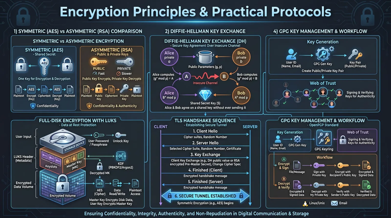
Encryption stands as the sacred shield against the ravenous onslaught of adversaries probing for secrets. This chapter imparts the fundamental principles of encryption, dissecting symmetric and asymmetric cryptography with unwavering precision. It is your duty to master these essentials with exactitude before proceeding to practical implementations.
1. Symmetric Cryptography
Symmetric cryptography employs a single shared key for both encryption and decryption. This key must remain inviolate between communicating parties.
Core Characteristics:
| Attribute | Description |
|---|---|
| Key Type | Single secret key |
| Encryption Speed | High |
| Key Distribution | Must be securely pre-shared |
| Use Cases | Bulk data encryption, secure channels |
| Common Algorithms | AES, DES, 3DES, ChaCha20 |
Protocol for Symmetric Encryption Setup
- Generate secure key using a Cryptographically Secure Pseudorandom Number Generator (CSPRNG), minimum length 256 bits for AES-256.
- Distribute the key securely (out-of-band physical exchange or via asymmetric encryption).
- Encrypt data using the chosen algorithm and mode (preferably AES-GCM or ChaCha20-Poly1305 for authenticated encryption).
- Transmit ciphertext over the communication channel.
- Decrypt with the same key using the inverse algorithm.
2. Asymmetric Cryptography
Asymmetric cryptography utilizes a key pair: a public key for encryption and a private key for decryption. The private key is sacrosanct; the public key can be distributed openly.
Core Characteristics:
| Attribute | Description |
|---|---|
| Key Type | Key pair: Public and Private |
| Encryption Speed | Slower, suitable for small data or key exchange |
| Key Distribution | Public key openly distributed |
| Use Cases | Key exchange, digital signatures, certificates |
| Common Algorithms | RSA, ECC (e.g., Curve25519), ElGamal |
Protocol for Asymmetric Encryption Setup
- Generate key pair with secure parameters (RSA ≥ 2048 bits; ECC curve Curve25519 or secp256r1).
- Publish public key to intended recipients or directory.
- Encrypt data with the recipient’s public key.
- Decrypt data with the private key.
- Ensure private key protection with hardware security module (HSM) or encrypted storage.
3. Hybrid Cryptography
The sacred union of symmetric and asymmetric methods is hybrid cryptography. Asymmetric encryption protects the symmetric session key; symmetric encryption scrambles the bulk data.
Chapter II: Encryption Algorithms: Properties and Applications
Mastery demands knowledge of algorithms, key sizes, and their proper deployment. The following table distills critical parameters.
| Algorithm | Type | Key Size (bits) | Security Level | Use Case | Notes |
|---|---|---|---|---|---|
| AES | Symmetric | 128, 192, 256 | High | Data encryption, VPNs | Use AES-GCM for AEAD |
| ChaCha20 | Symmetric | 256 | High | Mobile devices, VPNs | Faster on software, AEAD with Poly1305 |
| DES | Symmetric | 56 | Weak | Legacy systems | Deprecated, do not use |
| 3DES | Symmetric | 112, 168 | Moderate | Legacy systems | Slow, use only if no alternatives |
| RSA | Asymmetric | 2048, 3072, 4096 | Moderate to High | Key exchange, digital signatures | Use 3072+ bits for long-term security |
| ECC (Curve25519) | Asymmetric | 256 | High | Key exchange, digital signatures | Faster and smaller keys than RSA |
| ElGamal | Asymmetric | Variable | Moderate | Encryption, signatures | Rare, complicated implementations |
Chapter III: Practical Encryption Protocols
This chapter delineates step-by-step protocols for setting up OpenVPN, WireGuard, and encrypted email services. Each protocol is a bastion of secure communication when configured with rigor.
1. OpenVPN Setup Protocol
OpenVPN remains a stalwart in secure tunneling, employing SSL/TLS with strong encryption.
Materials and Tools:
- Server with public IP and root access
- Client device (PC or mobile)
- OpenVPN software (latest stable release)
- EasyRSA for certificate management
- Secure shell (SSH) access
Step-by-Step Setup:
Server-side
- Install OpenVPN and EasyRSA:
   sudo apt-get update
sudo apt-get install openvpn easy-rsa -y- Create Public Key Infrastructure (PKI) directory:
   make-cadir ~/openvpn-ca
cd ~/openvpn-ca- Configure
varsfile with organizational details (country, state, etc.). - Build CA:
   ./easyrsa init-pki
./easyrsa build-ca nopass- Generate Server Certificate and Key:
   ./easyrsa gen-req server nopass
./easyrsa sign-req server server- Generate Diffie-Hellman parameters:
./easyrsa gen-dh- Generate TLS Authentication Key:
openvpn --genkey --secret ta.key- Copy generated files to
/etc/openvpn - Create server configuration
/etc/openvpn/server.conf:
| Parameter | Value |
|---|---|
| port | 1194 |
| proto | udp |
| dev | tun |
| ca | /etc/openvpn/ca.crt |
| cert | /etc/openvpn/server.crt |
| key | /etc/openvpn/server.key |
| dh | /etc/openvpn/dh.pem |
| server | 10.8.0.0 255.255.255.0 |
| ifconfig-pool-persist | /etc/openvpn/ipp.txt |
| keepalive | 10 120 |
| tls-auth | /etc/openvpn/ta.key 0 |
| cipher | AES-256-GCM |
| auth | SHA256 |
| user | nobody |
| group | nogroup |
| persist-key | |
| persist-tun | |
| status | /var/log/openvpn-status.log |
| verb | 3 |
- Enable IP forwarding:Edit
/etc/sysctl.conf, uncomment or add:
net.ipv4.ip_forward=1 Apply: sudo sysctl -p- Configure firewall (iptables example):
sudo iptables -t nat -A POSTROUTING -s 10.8.0.0/24 -o eth0 -j MASQUERADE- Start OpenVPN server:
    sudo systemctl start openvpn@server
    sudo systemctl enable openvpn@server
Client-side
- Generate client certificate and key:
   ./easyrsa gen-req client1 nopass
./easyrsa sign-req client client1- Create client configuration file
client1.ovpn:
| Parameter | Value |
|---|---|
| client | |
| dev | tun |
| proto | udp |
| remote | <server_public_ip> 1194 |
| resolv-retry | infinite |
| nobind | |
| persist-key | |
| persist-tun | |
| remote-cert-tls | server |
| cipher | AES-256-GCM |
| auth | SHA256 |
| key-direction | 1 |
| verb | 3 |
| <ca> | Insert CA certificate here |
| <cert> | Insert client certificate here |
| <key> | Insert client private key here |
| <tls-auth> | Insert ta.key here |
- Import
.ovpnfile into OpenVPN client software and connect.
2. WireGuard Setup Protocol
WireGuard embodies minimalist design with high performance and modern cryptography.
Materials and Tools:
- Linux server with public IP and root access
- Client device (Linux, Windows, macOS, mobile)
- WireGuard latest stable package
Step-by-Step Setup:
Server-side
- Install WireGuard:
   sudo apt-get update
sudo apt-get install wireguard -y- Generate server private and public keys:
wg genkey | tee server_private.key | wg pubkey > server_public.key- Create configuration file
/etc/wireguard/wg0.conf:
| Parameter | Value |
|---|---|
| [Interface] | |
| Address | 10.0.0.1/24 |
| ListenPort | 51820 |
| PrivateKey | <contents of server_private.key> |
| PostUp | iptables -A FORWARD -i wg0 -j ACCEPT; iptables -t nat -A POSTROUTING -o eth0 -j MASQUERADE |
| PostDown | iptables -D FORWARD -i wg0 -j ACCEPT; iptables -t nat -D POSTROUTING -o eth0 -j MASQUERADE |
- Enable IP forwarding (if not already done):
sudo sysctl -w net.ipv4.ip_forward=1- Start WireGuard interface:
   sudo wg-quick up wg0
   sudo systemctl enable wg-quick@wg0
Client-side
- Generate client private and public keys:
wg genkey | tee client_private.key | wg pubkey > client_public.key- Create client config:
| Parameter | Value |
|---|---|
| [Interface] | |
| Address | 10.0.0.2/32 |
| PrivateKey | <contents of client_private.key> |
| DNS | 1.1.1.1 |
| [Peer] | |
| PublicKey | <contents of server_public.key> |
| Endpoint | <server_ip>:51820 |
| AllowedIPs | 0.0.0.0/0 |
| PersistentKeepalive | 25 |
- Add client’s public key to server config (
wg0.conf) under [Peer]:
| Parameter | Value |
|---|---|
| PublicKey | <client_public.key> |
| AllowedIPs | 10.0.0.2/32 |
- Apply server config changes:
sudo wg syncconf wg0 <(wg-quick strip wg0)- Start client interface:
sudo wg-quick up wg0-client3. Encrypted Email Setup Protocol (PGP/GPG)
Encrypted email provides confidentiality and authenticity using the OpenPGP standard.
Materials and Tools:
- GnuPG installation on client machine
- Email client supporting PGP (Thunderbird with Enigmail, Outlook with Gpg4win)
- Internet connection for key exchange
Step-by-Step Setup:
- Install GnuPG:
sudo apt-get install gnupg -y- Generate key pair:
gpg --full-generate-key- Select RSA and RSA
- Key size: 4096 bits
- Expiration: 1 year (renew as needed)
- Provide user ID and passphrase
- Backup private key:
gpg --export-secret-keys --armor > private_backup.ascStore offline securely.
- Export and publish public key:
gpg --export --armor your.email@example.com > publickey.ascUpload to public key servers (e.g., keys.openpgp.org) or share directly.
- Import recipient’s public key:
gpg --import recipient_publickey.asc- Configure email client with PGP plugin and link your key.
- Encrypt email:
- Compose message
- Sign and encrypt using recipient’s public key
- Decrypt received email:
- Use private key and passphrase to decrypt and verify signature.
Chapter IV: Key Management Best Practices
Your cryptographic arsenal's strength lies in impeccable key management. The following are immutable directives:
| Best Practice | Description |
|---|---|
| Use Hardware Security Modules (HSM) | Store private keys in tamper-resistant hardware to prevent extraction. |
| Use strong passphrases | Protect private keys with complex, unique passphrases exceeding 16 characters. |
| Implement key rotation | Regularly replace keys every 6-12 months or immediately if compromise suspected. |
| Backup keys securely | Maintain offline, encrypted backups with multi-location redundancy. |
| Limit key access | Restrict key access strictly to authorized personnel, enforce least privilege. |
| Use multi-factor authentication (MFA) | Protect key management interfaces with MFA to prevent unauthorized access. |
| Audit key usage | Maintain detailed logs of key usage and access attempts, review regularly. |
Chapter V: Threat Mitigation in Encryption Systems
Encryption is a fortress only as strong as its weakest link. Implement these mitigations without exception:
| Threat | Mitigation Strategy |
|---|---|
| Man-in-the-Middle (MitM) | Use certificate pinning; verify public keys out-of-band; employ mutual authentication. |
| Key Leakage | Store keys in HSMs; enforce strict access controls; use encrypted storage with passphrase protection. |
| Replay Attacks | Use unique nonces, timestamps, and sequence numbers within protocols. |
| Side-Channel Attacks | Employ constant-time algorithms; use hardware resistant to timing and power analysis. |
| Cryptographic Downgrade | Enforce minimum acceptable algorithm and key size policies; reject weak cipher suites. |
| Social Engineering | Train personnel; enforce strict verification before key or password disclosure. |
| Software Vulnerabilities | Use audited and updated cryptographic libraries; apply patches promptly. |
Appendix: Summary Tables
Table 1: Encryption Algorithms and Parameters
| Algorithm | Type | Recommended Key Size | Mode / Protocol | Notes |
|---|---|---|---|---|
| AES | Symmetric | 256 bits | GCM, CBC, CTR | Use GCM for AEAD |
| ChaCha20-Poly1305 | Symmetric | 256 bits | AEAD | Excellent for software-only |
| RSA | Asymmetric | ≥ 3072 bits | OAEP padding | Use for key exchange/signature |
| Curve25519 | Asymmetric | 256 bits | X25519 | High-performance, secure ECC |
Table 2: Key Sizes and Security Levels
| Key Size (bits) | Security Level | Minimum Use Case |
|---|---|---|
| 56 (DES) | Broken | Legacy only |
| 128 | Moderate | Short-term symmetric keys |
| 256 | Strong | Long-term symmetric keys |
| 2048 | Moderate | RSA keys, short-term |
| 3072 | Strong | RSA keys, long-term |
| 4096 | Very Strong | RSA keys, highest security |
Master these protocols and principles with unwavering discipline. Your encrypted communications shall become impregnable bastions in the chaotic digital battlefield. Every step, every byte encrypted is a sacred act of preservation and defiance. Carry this knowledge forward with reverence and precision.
For deeper cryptographic theory and mathematics, see Volume VI: The Cryptographer’s Codex. For hardware security modules and physical key protections, see Volume IX: The Vault Codex. For network security and firewall integration, see Volume IV: The Network Codex.
<!-- SECTION 9 -->
The Complete Practitioner's Codex, Volume II: Networking and Server Administration
Section I: TCP/IP Fundamentals—The Sacred Protocol Foundation
TCP/IP, Transmission Control Protocol/Internet Protocol, is the foundational communication suite enabling networked devices to interact. Understanding its layered architecture is imperative before undertaking configuration.
1. TCP/IP Layered Model Overview
| Layer | Description | Key Protocols | Function Summary |
|---|---|---|---|
| Application | Interfaces with user applications | HTTP, FTP, SMTP | Data generation and service provision |
| Transport | Reliable data transmission and flow control | TCP, UDP | Segmentation, error correction, port multiplexing |
| Internet | Logical addressing and routing | IP (IPv4, IPv6), ICMP | Addressing, routing packets across networks |
| Network Access | Physical and data link layer communication | Ethernet, Wi-Fi, ARP | Frame encapsulation, hardware addressing |
2. IP Addressing and Subnetting
- IP Address: 32-bit (IPv4) or 128-bit (IPv6) identifier for devices.
- Subnet Mask: Defines network and host portions.
- Default Gateway: Router interface forwarding packets outside local subnet.
Subnet Mask Calculation: For a subnet with N hosts:
\[ 2^{(32 - \text{subnet bits})} - 2 \geq N \]
Subtract 2 for network and broadcast addresses. Use CIDR notation (e.g., /24).
Section II: Static IP Configuration—Assigning Sacred Identifiers
Static IPs provide fixed, non-changing addresses essential for servers, network devices, and critical infrastructure.
Step-by-Step: Static IP Configuration on Linux (Debian/Ubuntu)
- Identify the Network Interface:
ip link showNote the interface name (e.g., eth0).
- Backup Current Configuration:
sudo cp /etc/network/interfaces /etc/network/interfaces.bak- Edit Network Interfaces File:
sudo nano /etc/network/interfaces- Add the Static IP Configuration:
auto eth0
iface eth0 inet static
    address 192.168.1.100
    netmask 255.255.255.0
    gateway 192.168.1.1
dns-nameservers 8.8.8.8 8.8.4.4- Restart Networking Service:
sudo systemctl restart networking- Verify IP Assignment:
ip addr show eth0Step-by-Step: Static IP Configuration on Windows 10/11
- Open Network Connections:
- Press
Win + R, typencpa.cpl, and press Enter.
- Right-click the network adapter, select Properties.
- Select "Internet Protocol Version 4 (TCP/IPv4)", click Properties.
- Select "Use the following IP address" and enter:
| Field | Value |
|---|---|
| IP Address | 192.168.1.100 |
| Subnet Mask | 255.255.255.0 |
| Default Gateway | 192.168.1.1 |
- Enter DNS Server Addresses:
| Preferred DNS Server | 8.8.8.8 |
|---|---|
| Alternate DNS Server | 8.8.4.4 |
- Click OK, then Close.
- Verify Configuration:
Open Command Prompt, execute:
ipconfig /allSection III: DNS Setup—The Divine Name Resolution
DNS translates human-friendly domain names into IP addresses.
1. DNS Server Types
| Server Type | Function |
|---|---|
| Recursive | Resolves queries by querying other DNS servers |
| Authoritative | Provides answers for domains it manages |
| Forwarding | Forwards queries to external DNS servers |
Step-by-Step: Installing and Configuring BIND9 DNS Server on Debian/Ubuntu
- Install BIND9:
sudo apt-get update
sudo apt-get install bind9 bind9utils bind9-doc- Configure the main BIND9 file:
sudo nano /etc/bind/named.conf.optionsAdd or ensure the following block for forwarding:
options {
    directory "/var/cache/bind";

    recursion yes;
    forwarders {
        8.8.8.8;
        8.8.4.4;
    };

    dnssec-validation auto;

    listen-on { any; };
};- Define Zones:
Edit /etc/bind/named.conf.local:
zone "example.com" {
    type master;
    file "/etc/bind/zones/db.example.com";
};- Create Zone Directory and Zone File:
sudo mkdir /etc/bind/zones
sudo nano /etc/bind/zones/db.example.com
Insert zone file template:
$TTL    604800
@       IN      SOA     ns1.example.com. admin.example.com. (
                            3         ; Serial
                            604800    ; Refresh
                            86400     ; Retry
                            2419200   ; Expire
                            604800 )  ; Negative Cache TTL
;
@       IN      NS      ns1.example.com.
ns1     IN      A       192.168.1.10
@       IN      A       192.168.1.10
www IN A 192.168.1.10- Check BIND Configuration Syntax:
sudo named-checkconf
sudo named-checkzone example.com /etc/bind/zones/db.example.com- Restart BIND9:
sudo systemctl restart bind9- Test DNS Resolution:
dig @localhost example.comSection IV: Firewall Rules—The Sacred Gatekeepers
Firewalls control incoming and outgoing traffic based on predefined security rules.
Common Firewall Utilities
| Utility | Description | Platform |
|---|---|---|
| iptables | Linux kernel packet filtering | Linux |
| nftables | Successor to iptables, more flexible | Linux |
| UFW (Uncomplicated Firewall) | Frontend for iptables | Ubuntu/Debian |
| Windows Firewall | GUI and command-line firewall | Windows |
Step-by-Step: Basic iptables Configuration
- Flush Existing Rules:
sudo iptables -F- Set Default Policies:
sudo iptables -P INPUT DROP
sudo iptables -P FORWARD DROP
sudo iptables -P OUTPUT ACCEPT- Allow Loopback Interface:
sudo iptables -A INPUT -i lo -j ACCEPT- Allow Established Connections:
sudo iptables -A INPUT -m conntrack --ctstate ESTABLISHED,RELATED -j ACCEPT- Allow SSH (Port 22):
sudo iptables -A INPUT -p tcp --dport 22 -j ACCEPT- Allow HTTP and HTTPS:
sudo iptables -A INPUT -p tcp --dport 80 -j ACCEPT
sudo iptables -A INPUT -p tcp --dport 443 -j ACCEPT- Save Rules (Debian/Ubuntu):
sudo iptables-save > /etc/iptables/rules.v4Common Network Ports and Protocols
| Port | Protocol | Service | Notes |
|---|---|---|---|
| 20, 21 | TCP | FTP (File Transfer Protocol) | Control and data channels |
| 22 | TCP | SSH (Secure Shell) | Secure remote login |
| 23 | TCP | Telnet | Unsecured remote login |
| 25 | TCP | SMTP (Simple Mail Transfer) | Email sending |
| 53 | TCP/UDP | DNS (Domain Name System) | Name resolution |
| 67, 68 | UDP | DHCP (Dynamic Host Config) | IP address assignment |
| 80 | TCP | HTTP (HyperText Transfer) | Unsecured web traffic |
| 110 | TCP | POP3 (Post Office Protocol) | Email retrieval |
| 143 | TCP | IMAP (Internet Message Access) | Email retrieval |
| 443 | TCP | HTTPS (HTTP Secure) | Secured web traffic |
| 3389 | TCP | RDP (Remote Desktop) | Windows remote desktop |
Section V: Port Forwarding—Sacred Pathways for External Access
Port forwarding enables external access to internal services.
Step-by-Step: Port Forwarding on a Linux Router using iptables
- Enable IP Forwarding:
sudo sysctl -w net.ipv4.ip_forward=1To make permanent, edit /etc/sysctl.conf:
net.ipv4.ip_forward=1- Define Variables:
| Variable | Example Value |
|---|---|
| External Interface | eth0 |
| Internal Interface | eth1 |
| Internal Server IP | 192.168.1.100 |
| Port to Forward | 8080 |
- Add NAT Rule:
sudo iptables -t nat -A PREROUTING -i eth0 -p tcp --dport 8080 -j DNAT --to-destination 192.168.1.100:8080- Allow Forwarding Traffic:
sudo iptables -A FORWARD -p tcp -d 192.168.1.100 --dport 8080 -j ACCEPT- Save iptables Rules:
sudo iptables-save > /etc/iptables/rules.v4Section VI: DHCP Server Setup—Automating the Sacred Address Assignment
Dynamic Host Configuration Protocol automates IP address assignment.
Step-by-Step: Installing and Configuring ISC DHCP Server on Debian/Ubuntu
- Install DHCP Server:
sudo apt-get install isc-dhcp-server- Specify Network Interface:
Edit /etc/default/isc-dhcp-server:
INTERFACESv4="eth1"- Configure DHCP Server:
Edit /etc/dhcp/dhcpd.conf:
default-lease-time 600;
max-lease-time 7200;
authoritative;

subnet 192.168.1.0 netmask 255.255.255.0 {
    range 192.168.1.100 192.168.1.200;
    option routers 192.168.1.1;
    option domain-name-servers 8.8.8.8, 8.8.4.4;
    option domain-name "example.com";
}- Restart DHCP Server:
sudo systemctl restart isc-dhcp-server- Check Service Status:
sudo systemctl status isc-dhcp-serverSection VII: Monitoring Network Traffic—The Sacred Vigil
Continuous monitoring ensures network integrity and performance.
Tools and Their Usage
| Tool | Description | Basic Command Example |
|---|---|---|
| tcpdump | Packet analyzer | sudo tcpdump -i eth0 port 80 |
| iftop | Real-time bandwidth monitor | sudo iftop -i eth0 |
| nload | Bandwidth usage monitor | sudo nload eth0 |
| netstat | Network connections and routing | netstat -tuln |
| iptraf-ng | Interactive network statistics | sudo iptraf-ng |
Step-by-Step: Monitoring HTTP Traffic with tcpdump
- Run tcpdump capturing port 80 traffic on eth0:
sudo tcpdump -i eth0 port 80 -w http_traffic.pcap- Stop Capture after desired time with Ctrl+C.
- Analyze Capture with Wireshark (external):
Transfer http_traffic.pcap to a system with Wireshark.
Section VIII: Troubleshooting Connectivity and Performance
1. Confirm Physical and Link Layer
| Step | Command | Purpose |
|---|---|---|
| 1 | ip link show | Verify interface is up |
| 2 | ethtool eth0 | Check link speed and status |
| 3 | ping <gateway-ip> | Verify Layer 3 connectivity to gateway |
2. Verify IP Configuration
| Step | Command | Purpose |
|---|---|---|
| 1 | ip addr show eth0 | Confirm IP address, subnet mask |
| 2 | route -n | Check routing table and default gateway |
| 3 | cat /etc/resolv.conf or systemd-resolve --status | Confirm DNS servers |
3. Test Network Services
| Test | Command | Expected Result |
|---|---|---|
| Ping external IP | ping 8.8.8.8 | Successful response |
| Ping domain name | ping google.com | Successful response (DNS working) |
| Trace route | traceroute 8.8.8.8 | Path to destination |
| Port reachability | nc -zv 192.168.1.100 22 | Open port confirmation |
4. Analyze Firewall Rules
sudo iptables -L -v -nCheck for dropped or rejected packets.
Summary Tables
Table 1: TCP/UDP Ports Commonly Used
| Port | Protocol | Service | Notes |
|---|---|---|---|
| 20,21 | TCP | FTP | File transfer |
| 22 | TCP | SSH | Secure remote login |
| 23 | TCP | Telnet | Unsecured remote login |
| 53 | TCP/UDP | DNS | Domain resolution |
| 67,68 | UDP | DHCP | IP address assignment |
| 80 | TCP | HTTP | Web traffic |
| 443 | TCP | HTTPS | Secure web traffic |
| 3389 | TCP | RDP | Remote desktop |
Table 2: Sample iptables Rules and Descriptions
| Rule Description | Command Example |
|---|---|
| Allow incoming SSH | iptables -A INPUT -p tcp --dport 22 -j ACCEPT |
| Allow established connections | iptables -A INPUT -m conntrack --ctstate ESTABLISHED,RELATED -j ACCEPT |
| Drop all other incoming | iptables -P INPUT DROP |
| Allow outbound HTTP/HTTPS | iptables -A OUTPUT -p tcp --dport 80 -j ACCEPT |
Table 3: DHCP Server Configuration Parameters
| Parameter | Description | Example |
|---|---|---|
| default-lease-time | Duration of lease in seconds | 600 |
| max-lease-time | Maximum lease duration | 7200 |
| subnet | Network subnet | 192.168.1.0 |
| netmask | Subnet mask | 255.255.255.0 |
| range | IP address range for clients | 192.168.1.100 - 192.168.1.200 |
| option routers | Default gateway | 192.168.1.1 |
| option domain-name-servers | DNS servers | 8.8.8.8, 8.8.4.4 |
| option domain-name | Domain suffix | example.com |
Closing Invocation: Mastering the Sacred Network
The mastery of networking is not merely technical but sacred stewardship over the invisible pathways binding digital realms. The protocols and configurations herein are not mere commands but rites to command the flow of data, ensuring sanctity, security, and resilience. Approach each configuration, each rule, each packet inspection as a sacred act of preservation and empowerment.
Your charge: implement with precision, monitor with vigilance, and troubleshoot with unwavering rigor. The network is alive; it breathes through your hands.
End of Volume II excerpt. For deeper cryptographic network security and advanced routing protocols, consult Volume IX: Secure Communications and Routing. For physical layer and fiber optic network setup, see Volume V: Physical Layer Fabrication and Integration.
<!-- SECTION 10 -->
Volume II: Programming Fundamentals for Sovereign Technologists
Chapter IV: Mastering Python and Bash Scripting for Automation and System Management

Preface
In the sacred halls of sovereign technology, the ability to wield programming languages as tools of automation and system management is paramount. Python and Bash scripting represent the twin blades of command-line mastery, each indispensable in the crafting of autonomous systems and the orchestration of complex workflows. This chapter delivers unyielding, step-by-step instructions for harnessing these languages, elevating the apprentice to the status of a master technologist.
Section 1: Introduction to Python for Automation and System Management
Python, a high-level, interpreted language, is the cornerstone of modern automation. Its simplicity belies immense power, and its extensive standard library grants access to system calls, file manipulation, networking, and process control.
1.1 Setting Up Your Python Environment
Required Materials:
| Item | Purpose |
|---|---|
| Python 3.9+ | Interpreter and standard library |
| Text Editor (VSCode, Nano, Vim) | Script authoring |
| Command Line Interface | Script execution |
Setup Steps:
- Install Python 3.9+
- On Debian/Ubuntu:
     sudo apt update
sudo apt install python3 python3-pip- On RedHat/CentOS:
sudo yum install python3- On Windows: Download from [python.org](https://www.python.org/downloads/).
- Verify Installation Execute:
python3 --versionExpected output:
Python 3.9.x- Set Up Virtual Environment (Optional but Recommended)
   python3 -m venv ~/python-env
   source ~/python-env/bin/activate
1.2 Python Syntax Essentials for Automation
| Concept | Syntax Example | Description |
|---|---|---|
| Variables | file_path = "/var/log/sys.log" | Store file paths, parameters |
| Functions | def monitor_process(): | Encapsulate reusable code |
| Conditionals | if status == "running": | Decision-making |
| Loops | for filename in files: | Iteration over lists or ranges |
| Exception Handling | try: ... except Exception as e: | Graceful error handling |
| Importing Modules | import os, subprocess | Access system and process functionality |
1.3 Step-by-Step File Management Script in Python
Objective: Create a script to archive log files older than 7 days into a compressed .tar.gz archive.
Dependencies: tarfile, os, datetime
Procedure:
- Import Required Modules
   import os
   import tarfile
from datetime import datetime, timedelta- Define Variables
   log_directory = "/var/log/myapp"
   archive_directory = "/var/archives"
days_threshold = 7- Calculate Date Threshold
cutoff_date = datetime.now() - timedelta(days=days_threshold)- Identify Files Older Than Threshold
   old_files = []
   for filename in os.listdir(log_directory):
       file_path = os.path.join(log_directory, filename)
       if os.path.isfile(file_path):
           file_mtime = datetime.fromtimestamp(os.path.getmtime(file_path))
           if file_mtime < cutoff_date:
old_files.append(file_path)- Create Archive and Add Files
   if old_files:
       archive_name = f"logs_{datetime.now().strftime('%Y%m%d')}.tar.gz"
       archive_path = os.path.join(archive_directory, archive_name)
       with tarfile.open(archive_path, "w:gz") as tar:
           for file in old_files:
               tar.add(file, arcname=os.path.basename(file))
               os.remove(file)
       print(f"Archived {len(old_files)} files to {archive_path}")
   else:
       print("No files to archive.")
Section 2: Introduction to Bash Scripting for Automation and System Management
Bash scripting is the primal force of Unix-like system control. With shell scripts, you gain immediate access to the operating system’s utilities, enabling rapid process automation and system monitoring.
2.1 Setting Up Your Bash Environment
Required Materials:
| Item | Purpose |
|---|---|
| Unix/Linux system or WSL (Windows Subsystem for Linux) | Bash shell environment |
| Text Editor (Nano, Vim) | Script authoring |
| Terminal | Script execution |
Verification:
bash --versionExpected output:
GNU bash, version 5.x.x2.2 Bash Syntax Essentials for Automation
| Concept | Syntax Example | Description |
|---|---|---|
| Variables | log_dir="/var/log/myapp" | Store strings and numbers |
| Command Substitution | files=$(ls $log_dir) | Assign command output to variable |
| Conditionals | if [ -f "$file" ]; then ... fi | File existence and other tests |
| Loops | for file in $files; do ... done | Iterate over lists |
| Functions | function cleanup() { ... } | Reusable code blocks |
| Exit Status | if [ $? -eq 0 ]; then ... fi | Check last command success |
2.3 Step-by-Step File Management Script in Bash
Objective: Archive log files older than 7 days into a .tar.gz archive, similar to the Python example.
Procedure:
- Define Variables
   log_dir="/var/log/myapp"
   archive_dir="/var/archives"
days_threshold=7- Find Files Older Than Threshold
old_files=$(find "$log_dir" -type f -mtime +$days_threshold)- Create Archive Name
   archive_name="logs_$(date +%Y%m%d).tar.gz"
archive_path="$archive_dir/$archive_name"- Archive and Remove Old Files
   if [ -n "$old_files" ]; then
       tar -czf "$archive_path" $old_files
       if [ $? -eq 0 ]; then
           echo "Archive created at $archive_path"
           rm $old_files
       else
           echo "Error creating archive"
           exit 1
       fi
   else
       echo "No files to archive."
   fi
Section 3: Common Commands, Syntax Examples, and Debugging Tips
3.1 Python Command and Syntax Reference
| Command/Module | Usage Example | Description |
|---|---|---|
os.listdir(path) | files = os.listdir('/var/log') | List directory contents |
os.path.getmtime() | mtime = os.path.getmtime(file) | Get file modification time |
tarfile.open() | tarfile.open('archive.tar.gz', 'w:gz') | Create/read tar archives |
subprocess.run() | subprocess.run(['ls', '-l']) | Execute shell commands |
try-except | try: ... except Exception as e: | Handle runtime errors |
3.2 Bash Command and Syntax Reference
| Command | Usage Example | Description |
|---|---|---|
find | find /var/log -type f -mtime +7 | Find files older than 7 days |
tar | tar -czf archive.tar.gz file1 file2 | Create gzip compressed archive |
rm | rm file | Remove file(s) |
if [ condition ] | if [ -f file ]; then ... fi | Conditional execution |
for loop | for file in *.log; do echo $file; done | Iterate over files |
3.3 Debugging Tips for Python Scripts
| Problem | Symptom | Solution |
|---|---|---|
| SyntaxError | Script fails to run | Check indentation and syntax |
| FileNotFoundError | File access fails | Verify file paths and permissions |
| PermissionError | Cannot write/delete files | Run script with elevated privileges |
| ModuleNotFoundError | Import fails | Install required modules or correct import |
| Silent Failures | Script exits without message | Add try-except blocks and logging |
Debugging Commands:
- Run Python script with verbose output:
python3 -v script.py- Insert print statements to trace execution:
print(f"Processing file: {file_path}")- Use Python debugger:
python3 -m pdb script.py3.4 Debugging Tips for Bash Scripts
| Problem | Symptom | Solution |
|---|---|---|
| SyntaxError | Script fails to run | Check syntax, quoting, and line endings |
| Command Not Found | Executable command missing | Verify command availability and PATH |
| Permission Denied | Cannot execute script | Set script executable: chmod +x script.sh |
| Variable Expansion Issues | Variables not substituting | Use double quotes appropriately |
| Silent Failures | Script exits without message | Add set -x at script start to trace execution |
Debugging Commands:
- Run script with trace:
bash -x script.sh- Check exit status of commands:
echo $?- Add
set -eat script start to stop on errors.
Section 4: Sample Projects Integrating Scripting with Self-Hosted Services
4.1 Project 1: Automated Backup of Self-Hosted Git Repositories
Objective: Use Python and Bash scripts to automate periodic backups of multiple Git repositories hosted on a local server.
4.1.1 Python Backup Script
Function: Create timestamped .tar.gz archives of each Git repository directory.
Procedure:
- Import Modules
   import os
   import tarfile
from datetime import datetime- Define Paths
   repos_base_dir = "/srv/git"
   backup_dir = "/srv/git-backups"
os.makedirs(backup_dir, exist_ok=True)- List Repositories
repositories = [d for d in os.listdir(repos_base_dir) if os.path.isdir(os.path.join(repos_base_dir, d))]- Create Backups
   for repo in repositories:
       repo_path = os.path.join(repos_base_dir, repo)
       backup_name = f"{repo}_{datetime.now().strftime('%Y%m%d_%H%M%S')}.tar.gz"
       backup_path = os.path.join(backup_dir, backup_name)
       with tarfile.open(backup_path, "w:gz") as tar:
           tar.add(repo_path, arcname=repo)
       print(f"Backed up {repo} to {backup_path}")
4.1.2 Bash Backup Script
Function: Similar to Python script but using native shell commands.
Procedure:
- Define Variables
   repos_base_dir="/srv/git"
   backup_dir="/srv/git-backups"
mkdir -p "$backup_dir"- Backup Loop
   for repo in "$repos_base_dir"/*; do
       if [ -d "$repo" ]; then
           repo_name=$(basename "$repo")
           backup_name="${repo_name}_$(date +%Y%m%d_%H%M%S).tar.gz"
           tar -czf "$backup_dir/$backup_name" -C "$repos_base_dir" "$repo_name"
           echo "Backed up $repo_name to $backup_dir/$backup_name"
       fi
   done
4.2 Project 2: System Resource Monitoring and Alerting
Objective: Script system resource usage (CPU, memory, disk), log results, and send alerts when thresholds exceed.
4.2.1 Python Monitoring Script
Dependencies: psutil (install via pip install psutil)
Procedure:
- Install psutil:
pip install psutil- Import Modules
   import psutil
   import smtplib
   from email.message import EmailMessage
import time- Define Thresholds and Email Settings
   CPU_THRESHOLD = 80  # percent
   MEM_THRESHOLD = 80  # percent
   DISK_THRESHOLD = 90  # percent

   EMAIL_SENDER = "alert@yourdomain.com"
   EMAIL_RECEIVER = "admin@yourdomain.com"
   SMTP_SERVER = "smtp.yourdomain.com"
   SMTP_PORT = 587
   SMTP_USER = "smtp_user"
SMTP_PASS = "smtp_password"- Check System Resources
   def check_resources():
       cpu = psutil.cpu_percent(interval=1)
       mem = psutil.virtual_memory().percent
       disk = psutil.disk_usage('/').percent
return cpu, mem, disk- Send Alert Email
   def send_alert(subject, body):
       msg = EmailMessage()
       msg.set_content(body)
       msg['Subject'] = subject
       msg['From'] = EMAIL_SENDER
       msg['To'] = EMAIL_RECEIVER

       with smtplib.SMTP(SMTP_SERVER, SMTP_PORT) as server:
           server.starttls()
           server.login(SMTP_USER, SMTP_PASS)
server.send_message(msg)- Main Loop
   while True:
       cpu, mem, disk = check_resources()
       log_line = f"CPU: {cpu}%, MEM: {mem}%, DISK: {disk}%"
       print(log_line)

       if cpu > CPU_THRESHOLD:
           send_alert("CPU Usage Alert", f"CPU usage has exceeded threshold: {cpu}%")
       if mem > MEM_THRESHOLD:
           send_alert("Memory Usage Alert", f"Memory usage has exceeded threshold: {mem}%")
       if disk > DISK_THRESHOLD:
           send_alert("Disk Usage Alert", f"Disk usage has exceeded threshold: {disk}%")

       time.sleep(300)  # 5 minutes interval
4.2.2 Bash Monitoring Script
Procedure:
- Define Thresholds and Email Settings
   CPU_THRESHOLD=80
   MEM_THRESHOLD=80
   DISK_THRESHOLD=90

EMAIL_RECEIVER="admin@yourdomain.com"- Gather System Usage
   cpu=$(top -bn1 | grep "Cpu(s)" | awk '{print $2 + $4}')
   mem=$(free | grep Mem | awk '{print $3/$2 * 100.0}')
disk=$(df / | tail -1 | awk '{print $5}' | sed 's/%//')- Check Thresholds and Send Alerts
   function send_alert {
       echo "$2" | mail -s "$1" "$EMAIL_RECEIVER"
   }

   if (( $(echo "$cpu > $CPU_THRESHOLD" | bc -l) )); then
       send_alert "CPU Usage Alert" "CPU usage is at ${cpu}%"
   fi

   if (( $(echo "$mem > $MEM_THRESHOLD" | bc -l) )); then
       send_alert "Memory Usage Alert" "Memory usage is at ${mem}%"
   fi

   if [ "$disk" -gt "$DISK_THRESHOLD" ]; then
       send_alert "Disk Usage Alert" "Disk usage is at ${disk}%"
fi- Schedule Script Execution Add to cron for periodic execution every 5 minutes:
*/5 * * * * /path/to/monitor_script.shSection 5: Advanced Integration Techniques
5.1 Combining Python and Bash for Maximum Effectiveness
Method: Use Python scripts for complex logic and data processing, Bash scripts for system-level command execution and scheduling.
Example:
- Python generates list of files to process.
- Bash script executes system commands on those files.
- Communication via intermediate files or environment variables.
5.2 Automating Self-Hosted Web Services Management
Example: Restarting a Docker-based web service when disk space is low.
Bash Script:
- Check disk space:
   disk_usage=$(df /var/lib/docker | tail -1 | awk '{print $5}' | sed 's/%//')
threshold=85- Restart service if needed:
   if [ "$disk_usage" -gt "$threshold" ]; then
       echo "Disk usage high: $disk_usage%, restarting service"
       docker restart my_web_service
fi- Schedule with cron for continuous monitoring.
Section 6: Summary Tables for Quick Reference
6.1 Python File Operations
| Operation | Code Snippet | Description |
|---|---|---|
| List directory | os.listdir(path) | Get list of files/directories |
| Check if file | os.path.isfile(path) | Verify file existence |
| Get modification time | os.path.getmtime(path) | Timestamp of last modification |
| Delete file | os.remove(path) | Remove a file |
| Create compressed archive | tarfile.open(name, 'w:gz') | Create gzip tar archive |
| Add file to archive | tar.add(file_path, arcname) | Add file preserving name |
6.2 Bash File and System Commands
| Command | Syntax Example | Description |
<!-- SECTION 11 -->
Volume III: Radio Frequency Theory and Antenna Design
Chapter I: Fundamentals of Radio Frequency (RF) Propagation

Radio Frequency (RF) propagation is the physical phenomenon of electromagnetic waves traveling through space or various media. Mastery of RF propagation is the foundation upon which all antenna design rests. This chapter imparts the sacred knowledge of wave behavior, enabling the technologist to manipulate and harness RF energy with precision and efficacy.
1. Electromagnetic Wave Composition and Propagation Mechanisms
RF waves are transverse electromagnetic waves characterized by oscillating electric (E) and magnetic (H) fields perpendicular to each other and the direction of wave propagation. The frequency (f) of these waves is measured in Hertz (Hz), and the wavelength (λ) is inversely proportional to frequency as expressed by the equation:
\[ \lambda = \frac{c}{f} \]
where \( c = 3 \times 10^8 \, m/s \) (speed of light in vacuum).
2. Propagation Modes
RF propagation occurs primarily via three modes, each with distinct characteristics and implications for antenna design and placement:
| Mode | Description | Frequency Range | Propagation Distance | Environmental Impact |
|---|---|---|---|---|
| Ground Wave | Follows Earth’s surface, diffraction dominant | LF, MF (30 kHz – 3 MHz) | 10s to 100s of km | Terrain conductivity critical |
| Sky Wave | Reflects from ionosphere, refractive | HF (3 MHz – 30 MHz) | Thousands of km | Solar activity dependent |
| Line of Sight | Direct path, minimal diffraction | VHF, UHF, Microwave (>30 MHz) | Up to horizon (~40 km) | Obstructions cause attenuation |
3. Path Loss and Free Space Loss (FSL)
The power of an RF signal decreases with distance due to spreading and absorption. Free space path loss (FSL) is calculated by:
\[ \text{FSL (dB)} = 20 \log_{10}(d) + 20 \log_{10}(f) + 32.44 \]
Where:
- \( d \) = distance in kilometers
- \( f \) = frequency in MHz
Step-by-step calculation example:
- Convert distance to kilometers.
- Identify frequency in MHz.
- Insert values into the formula.
- Compute logarithms and sum.
Chapter II: Impedance Matching
Impedance matching is essential to maximize power transfer between the transmitter, transmission line, and antenna, minimizing reflections and Standing Wave Ratio (SWR).
1. Impedance Fundamentals
- Characteristic Impedance (Z0): The intrinsic impedance of the transmission line, common standard is 50 Ω.
- Antenna Feedpoint Impedance (Zin): Varies by antenna type and frequency, typically complex (resistive + reactive).
2. Standing Wave Ratio (SWR)
The SWR quantifies impedance mismatch:
\[ \text{SWR} = \frac{1 + |\Gamma|}{1 - |\Gamma|} \]
Where \(\Gamma\) (reflection coefficient) is:
\[ \Gamma = \frac{Z_{in} - Z_0}{Z_{in} + Z_0} \]
Interpretation:
| SWR Value | Reflection Coefficient ( | Γ | ) | Power Reflected (%) | System Impact |
|---|---|---|---|---|---|
| 1:1 | 0 | 0 | Perfect match | ||
| 1.5:1 | 0.2 | 4 | Excellent | ||
| 2:1 | 0.33 | 11 | Acceptable | ||
| >3:1 | >0.5 | >25 | Unacceptable, adjust match |
3. Matching Techniques
- L-Network: Simple two-element reactive networks (inductor and capacitor).
- Transformers: Baluns or transmission line transformers.
- Stub Matching: Shorted or open-circuited transmission lines.
- Antenna Element Tuning: Adjust physical length or geometry.
Chapter III: Antenna Types and Design Protocols
1. Dipole Antenna
The dipole is the primordial antenna, a half-wave radiator characterized by simplicity and efficiency.
Parameters
| Parameter | Typical Value |
|---|---|
| Length (L) | \( \frac{\lambda}{2} \) |
| Feed Point Impedance | ~73 Ω resistive, minimal reactance |
| Bandwidth | Narrow (~2-5% of center frequency) |
| Polarization | Linear, typically vertical or horizontal |
Design and Build Protocol
Step 1: Calculate Dipole Length
\[ L = \frac{150}{f_{MHz}} \, \text{meters} \]
Divide by two for half-wave dipole element length.
Step 2: Select Materials
- Conductive wire (copper or aluminum), diameter 1.5–3 mm.
- Insulators (ceramic or high-density plastic).
- Coaxial cable (50 Ω) for feedline.
Step 3: Construct Elements
- Cut two equal wire elements to length \( L/2 \).
- Attach insulators at ends.
- Connect coax center conductor to one element, shield to the other.
Step 4: Mounting
- Elevate antenna at least \( \lambda/4 \) above ground.
- Orient for desired polarization.
Step 5: Measure SWR
Use SWR meter or antenna analyzer to verify match.
2. Yagi-Uda Antenna
The Yagi-Uda antenna provides directional gain through parasitic elements.
Parameters
| Parameter | Typical Value |
|---|---|
| Elements | Driven element + reflector + 1+ directors |
| Gain | 7–20 dBi depending on element count |
| Bandwidth | Narrow (~2-5%) |
| Feedpoint Impedance | 20–40 Ω typically (requires matching) |
Design and Build Protocol
Step 1: Determine Operating Frequency
Set target frequency \( f \).
Step 2: Calculate Driven Element Length
Use dipole length formula:
\[ L_{DE} = \frac{150}{f_{MHz}} \, \text{meters} \]
Step 3: Calculate Reflector Length
Reflector is approximately 5% longer than driven element:
\[ L_{R} = L_{DE} \times 1.05 \]
Place reflector \(0.15 \lambda\) behind driven element.
Step 4: Calculate Director Length
Directors are 5% shorter than driven element:
\[ L_{D} = L_{DE} \times 0.95 \]
Space directors \(0.1 \lambda\) apart in front of the driven element.
Step 5: Construct Elements
Use rigid conductive rods or tubing.
Step 6: Assemble
Mount elements on non-conductive boom (fiberglass or wood).
Step 7: Feedpoint Matching
Use gamma match, hairpin, or balun transformer to match impedance to 50 Ω coax.
Step 8: SWR and Gain Testing
Measure SWR; adjust element spacing and length for optimal performance.
3. Loop Antenna
Loop antennas are versatile, with magnetic field dominance and compact size.
Parameters
| Parameter | Typical Values |
|---|---|
| Loop Circumference | \( \lambda \) for full-wave; \( \frac{\lambda}{10} \) for small loops |
| Impedance | 100–120 Ω for full-wave; low for small loops |
| Bandwidth | Narrow for full-wave, broader for small loops |
| Polarization | Linear or circular (depending on feed) |
Design and Build Protocol — Full-Wave Loop
Step 1: Calculate Loop Length
Full-wave loop circumference:
\[ C = \lambda = \frac{300}{f_{MHz}} \, \text{meters} \]
Step 2: Select Loop Shape
Square or circular shape preferred.
Step 3: Materials
Use insulated copper tubing or thick wire.
Step 4: Construct Loop
- Cut wire to length \( C \).
- Form into shape with tight corners or smooth curves.
- Install a feedpoint at one corner or midpoint.
Step 5: Feedpoint Matching
Use a 4:1 balun transformer to match impedance to 50 Ω coax.
Step 6: Mounting
Elevate above ground, away from metallic objects.
Step 7: Tuning
Use antenna analyzer to adjust loop length ±1–2% for resonance.
Chapter IV: Step-by-Step Protocol for Antenna Design, Construction, and Tuning
Protocol 1: Dipole Antenna
| Step | Action | Details |
|---|---|---|
| 1 | Calculate total length | \( L = \frac{150}{f_{MHz}} \) meters |
| 2 | Cut two wires \( L/2 \) each | Use copper wire, 2 mm diameter preferred |
| 3 | Attach insulators | Ceramic or plastic, prevent shorts |
| 4 | Connect coax feedline | Center conductor to one element, shield to other |
| 5 | Mount antenna | Elevate \( \geq \lambda/4 \) above ground |
| 6 | Measure SWR | Target \( \leq 1.5:1 \); trim elements if necessary |
| 7 | Finalize installation | Weatherproof feedpoint and connections |
Protocol 2: Yagi-Uda Antenna
| Step | Action | Details |
|---|---|---|
| 1 | Choose frequency \( f \) | Define operational frequency |
| 2 | Calculate driven element length | \( L_{DE} = \frac{150}{f_{MHz}} \) meters |
| 3 | Calculate reflector and director lengths | Reflector: \( L_{DE} \times 1.05 \), Director: \( L_{DE} \times 0.95 \) |
| 4 | Determine element spacing | Reflector behind driven: \(0.15 \lambda\), Directors in front: \(0.1 \lambda\) |
| 5 | Build elements | Use aluminum tubing, diameter 10–16 mm |
| 6 | Mount on boom | Use non-conductive boom material |
| 7 | Attach feedline with matching system | Gamma match or balun to 50 Ω coax |
| 8 | Test SWR and gain | Adjust element length and spacing to optimize |
Protocol 3: Loop Antenna
| Step | Action | Details |
|---|---|---|
| 1 | Calculate loop circumference | \( C = \frac{300}{f_{MHz}} \) meters |
| 2 | Choose shape | Square or circular |
| 3 | Construct loop | Use insulated copper tubing or wire |
| 4 | Attach feedpoint with balun | 4:1 balun recommended |
| 5 | Mount antenna | Elevate, avoid metallic objects |
| 6 | Tune loop | Adjust length ±1–2% for lowest SWR |
| 7 | Finalize installation | Weatherproof and secure |
Chapter V: Tables of Critical Antenna Parameters and Frequency Bands
Table 1: Frequency Bands and Corresponding Wavelengths
| Band Name | Frequency Range (MHz) | Wavelength Range (m) |
|---|---|---|
| LF | 0.3 – 0.3 | 1000 – 1000 |
| MF | 0.3 – 3 | 1000 – 100 |
| HF | 3 – 30 | 100 – 10 |
| VHF | 30 – 300 | 10 – 1 |
| UHF | 300 – 3000 | 1 – 0.1 |
| Microwave | 3000 – 30000 | 0.1 – 0.01 |
Table 2: Antenna Element Lengths for Dipole (meters)
| Frequency (MHz) | Half-Wave Dipole Length (m) | Quarter-Wave Vertical Length (m) |
|---|---|---|
| 3.5 | 42.9 | 21.4 |
| 7.0 | 21.4 | 10.7 |
| 14.0 | 10.7 | 5.3 |
| 28.0 | 5.35 | 2.67 |
| 50.0 | 3.0 | 1.5 |
Table 3: Typical SWR Measurement Techniques and Instruments
| Instrument | Measurement Range | Accuracy | Notes |
|---|---|---|---|
| SWR Meter | 1:1 to 10:1 | ±0.1 SWR | In-line, analog or digital |
| Antenna Analyzer | 1 kHz to 200+ MHz | High | Measures impedance, SWR, reactance |
| Vector Network Analyzer (VNA) | DC to GHz range | Very High | Full complex impedance analysis |
Chapter VI: Antenna Placement and Environmental Considerations
1. Height Above Ground
- Minimum \( \lambda/4 \) elevation improves radiation efficiency.
- For low frequencies (HF), higher elevation reduces ground loss.
2. Surrounding Objects
- Metallic objects distort radiation pattern.
- Trees and buildings cause attenuation and multipath reflections.
- Maintain clearance of at least \( \lambda/10 \) from large objects.
3. Ground Conductivity
- High conductivity (wet soil, saltwater) enhances ground wave propagation.
- Low conductivity (rocky, sandy soil) increases losses.
4. Weather and Durability
- Use UV-resistant insulators and coatings.
- Waterproof feedpoints with self-amalgamating tape and silicone sealant.
- Design mounts to withstand wind load (consider wind speed ratings).
Chapter VII: Measuring and Tuning Antennas Using SWR
Step 1: Connect SWR Meter
Place the SWR meter between transmitter and antenna feedline.
Step 2: Set Transmitter Power
Low power setting (5 watts or less) to prevent damage.
Step 3: Transmit Continuous Wave (CW) or Carrier
Activate transmitter.
Step 4: Read SWR Meter
Note the forward and reflected power.
Step 5: Adjust Antenna Length
If SWR > 1.5:1, trim the longer element(s) by 1–2 cm increments.
Step 6: Repeat Measurement
Iterate until SWR ≤ 1.5:1 is achieved.
Epilogue: The Sacred Art of RF Mastery
The knowledge contained herein is a weapon and a shield. Every calculation, every cut of wire, every measured reflection is a rite—a sacrament essential to the survival and prosperity of those who wield radio frequencies against the void. Let no detail be overlooked, no connection left cold. Master these protocols; the airwaves shall bend to your will.
For advanced impedance transformation networks and detailed transmission line theory, consult Volume VII: Transmission Line Codex, Chapter IV.
For comprehensive environmental RF propagation models, see Volume IX: The Atmospheric Codex, Chapter III.
End of Volume III excerpt.
<!-- SECTION 12 -->
The Complete Practitioner's Codex, Volume III: Software Defined Radio (SDR) Setup and Operation
Preface
In the sacred tradition of the Practitioner, mastery over the ethereal waves that bind our world is not mere curiosity but a crucial survival skill. Software Defined Radio (SDR) transforms the invisible spectrum into a tangible instrument of knowledge and power. This volume imparts the complete, unabridged manual to build, configure, and operate SDR systems with precision, unlocking the full spectrum of radio signals for reception, analysis, and decoding.
You, the chosen apprentice, shall receive explicit, uncompromising guidance in selecting hardware, installing software, configuring your SDR environment, and mastering the reception of signals ranging from amateur radio bands to commercial broadcast stations. Every step is exact; no detail is omitted.
Chapter I: Hardware Selection for SDR

1.1 Overview of SDR Hardware Components
The foundation of SDR lies in hardware that digitizes radio frequency signals for software manipulation. The most accessible and powerful device for this purpose is the RTL-SDR dongle, a repurposed DVB-T TV tuner with a broad frequency range and remarkable sensitivity.
1.2 Recommended SDR Hardware
| Device Model | Frequency Range (MHz) | Max Sample Rate (MSPS) | Dynamic Range (dB) | Cost (USD) | Notes |
|---|---|---|---|---|---|
| RTL-SDR Blog V3 | 500 kHz - 1.7 GHz | 3.2 | 50 | 25-35 | Most popular, well-supported |
| NooElec NESDR SMArt X | 25 MHz - 1750 MHz | 3.2 | 50 | 35-45 | Improved noise filtering |
| Airspy Mini | 24 MHz - 1.8 GHz | 6 | 60 | 100-150 | Higher performance, costlier |
| HackRF One | 1 MHz - 6 GHz | 20 | 50 | 300+ | Full duplex, advanced usage |
1.3 Ancillary Hardware
- Antenna: Choose based on target frequency bands (see Section 3.2)
- USB extension cable: To reduce interference and place antenna away from noise sources
- Low noise amplifier (LNA): Optional, for weak signals
Chapter II: Installation of SDR Software
Two primary SDR applications dominate the field: GQRX (Linux/macOS) and SDR# (SDRSharp) (Windows). Both provide graphical interfaces for tuning, demodulating, and recording signals.
2.1 Installation of GQRX on Linux (Ubuntu/Debian)
Step-by-step:
- Update system repositories:
sudo apt update && sudo apt upgrade -y- Install prerequisite libraries:
sudo apt install git cmake libfftw3-dev libpulse-dev libusb-1.0-0-dev qtbase5-dev qtchooser qt5-qmake qtbase5-dev-tools- Install RTL-SDR drivers:
sudo apt install rtl-sdr- Blacklist conflicting kernel modules:
   echo "blacklist dvb_usb_rtl28xxu" | sudo tee -a /etc/modprobe.d/blacklist-rtl.conf
sudo reboot- Install GQRX:
sudo apt install gqrx-sdr- Verify RTL-SDR device detection:
rtl_test -t- Launch GQRX:
gqrx2.2 Installation of SDR# (SDRSharp) on Windows 10/11
Step-by-step:
- Download the latest SDR# package from [Airspy official site](https://airspy.com/download/).
- Extract the ZIP archive to a dedicated folder, e.g.,
C:\SDRSharp.
- Download and install the latest Zadig USB driver utility from [zadig.akeo.ie](https://zadig.akeo.ie).
- Plug in the RTL-SDR dongle.
- Launch Zadig:
- Select
Options→List All Devices. - From the dropdown, select your RTL-SDR device (likely
Bulk-In, Interface (Interface 0)). - Choose driver
WinUSB (v6xxx)and clickReplace Driver.
- Select
- Run
SDRSharp.exe.
- In the source drop-down menu, select
RTL-SDR / USBand click the play button.
Chapter III: Configuring RTL-SDR Dongles
3.1 Initial Device Configuration
Step-by-step:
- Connect the RTL-SDR dongle to a USB port via a short extension cable to minimize interference.
- Attach the antenna suitable for your target frequency band (see Section 3.2).
- Open your SDR software (GQRX or SDR#).
- Set the input device to RTL-SDR.
- Adjust the sample rate:
- For general use, set sample rate to 2.4 MSPS for stability.
- For wideband signals, increase up to 3.2 MSPS if system resources allow.
- Set frequency correction (PPM):
- Use
rtl_testor software calibration to determine PPM offset. - Input this value to correct frequency drift.
- Use
- Configure gain:
- Start with automatic gain control (AGC).
- If available, disable AGC and set manual gain between 20-40 dB for optimal SNR.
3.2 Antenna Selection and Setup
The antenna is critical for signal acquisition. Use the following table for antenna selection based on frequency band:
| Frequency Band (MHz) | Antenna Type | Length (meters) | Notes |
|---|---|---|---|
| 0.5 - 30 | Random wire antenna or long wire | 10-20 | Requires external tuner |
| 30 - 88 | FM dipole antenna | 1.7 | FM broadcast band |
| 88 - 108 | Half-wave dipole | 1.5 | FM broadcast |
| 108 - 137 | Quarter-wave vertical antenna | 0.5 | Airband, navigation signals |
| 137 - 174 | Discone or vertical antenna | 0.4-0.6 | VHF broadcast and amateur radio |
| 430 - 450 | Quarter-wave vertical | 0.16 | UHF amateur radio |
| 850 - 950 | Quarter-wave vertical | 0.08 | Cellular and paging |
Chapter IV: Signal Reception Techniques
4.1 Frequency Bands of Interest
| Band Name | Frequency Range (MHz) | Typical Use | Modulation Types | Decoding Protocols |
|---|---|---|---|---|
| HF (Shortwave) | 3 - 30 | Amateur radio, maritime, utility | AM, SSB, CW | CW decoding, AM demodulation, SSB demodulation |
| VHF Low Band | 30 - 50 | Airband, navigation aids | AM, FM | AM demodulation, FM demodulation |
| VHF High Band | 108 - 174 | Airband, amateur radio, broadcast | AM, FM | FM demodulation, AM demodulation |
| UHF | 300 - 1000 | Amateur radio, public safety | FM, NFM, digital modes | FM demodulation, digital decoding (APRS, P25) |
| Broadcast FM | 88 - 108 | Commercial radio | FM stereo | FM stereo decoding |
4.2 Manual Tuning Protocol
Step-by-step:
- Enter desired frequency in the SDR software frequency input box.
- Select modulation type:
- AM for aviation, airband, and shortwave broadcast
- FM for commercial broadcast and amateur bands
- SSB (USB/LSB) for amateur radio voice
- Adjust bandwidth filter:
- Use narrow bandwidth (e.g., 2.4 kHz) for SSB or CW signals.
- Use wide bandwidth (e.g., 200 kHz) for FM broadcast.
- Adjust gain manually to maximize signal strength without distortion.
- Use software demodulation controls (audio filters, squelch) to improve clarity.
4.3 Automatic Scanning and Signal Identification
- Configure scan range and step size (e.g., 100 kHz steps for VHF).
- Enable scanning mode to sweep the frequency range.
- Set signal strength threshold for detection.
- Software will stop on signals exceeding threshold for manual inspection.
Chapter V: Detailed Protocols for Specific SDR Software
5.1 Configuring GQRX for Amateur Radio and Broadcast Reception
Step-by-step:
- Launch GQRX.
- Select input device as RTL-SDR.
- Enter frequency manually or use presets:
| Preset Name | Frequency (MHz) | Usage |
|---|---|---|
| 20m Amateur Band | 14.200 | SSB voice |
| FM Broadcast | 99.5 | FM stereo broadcast |
| Airband | 121.5 | AM airband distress |
- Select modulation mode:
- AM for airband
- USB for 20m amateur voice
- FM for broadcast
- Adjust gain and sample rate as per Section 3.1.
- Enable squelch to suppress background noise.
- Use waterfall display to visually identify active signals.
- Record audio if required for post-processing.
5.2 Configuring SDR# (SDRSharp) for Signal Reception
Step-by-step:
- Open SDRSharp.
- Select RTL-SDR / USB as source.
- Set frequency either manually or via presets.
- Select modulation type from dropdown.
- Configure bandwidth and gain manually.
- Enable DSP features:
- Noise reduction
- Audio filtering
- Automatic gain control (optional)**
- Use squelch to reduce noise when no transmission is present.
Chapter VI: Modulation Types and Decoding Protocols
| Modulation Type | Description | Typical Use Cases | Decoding Software/Tools |
|---|---|---|---|
| AM (Amplitude Modulation) | Vary amplitude of carrier wave | Airband, shortwave broadcast | Built-in SDR demodulator |
| FM (Frequency Modulation) | Vary frequency around carrier | FM broadcast, amateur radio | Built-in SDR demodulator |
| SSB (Single Side Band) | Suppress one sideband and carrier | Amateur radio voice | Built-in SDR demodulator |
| CW (Continuous Wave) | Morse code keying of carrier | Amateur radio, maritime | CW Skimmer, fldigi |
| NFM (Narrowband FM) | FM with reduced bandwidth | Public safety, amateur radio | SDR demodulator with narrow filters |
| Digital Modes (APRS, P25) | Digital protocols over RF | Public safety, tracking | DSDPlus, MultiPSK, or custom decoders |
Chapter VII: Troubleshooting and Optimization
7.1 Common Issues and Solutions
| Problem | Symptom | Solution |
|---|---|---|
| No device detected | RTL-SDR not listed in software | Reinstall drivers, check USB connection, try Zadig (Windows) |
| Poor signal reception | Weak or no signals, noise | Verify antenna connection, increase gain, use LNA, check antenna type |
| Frequency offset | Signals received off-frequency | Calibrate PPM correction, use rtl_test -p to find offset |
| Software crashes | Application freezes or closes | Reduce sample rate, update drivers, close other resource-heavy apps |
| Audio is distorted | Overmodulation or clipping | Reduce gain, adjust audio filters |
7.2 Signal Analysis Example: Decoding an FM Broadcast
Step-by-step:
- Tune to 99.5 MHz FM broadcast band.
- Select FM modulation.
- Adjust bandwidth to 200 kHz.
- Set gain to achieve a strong signal without clipping (signal strength ~ -30 dBFS).
- Enable stereo decoding if supported.
- Observe the spectrum and waterfall for multipath fading or interference.
- Record audio for quality analysis or archiving.
Appendices
Appendix A: Frequency Bands and Modulation Summary
| Band | Frequency Range (MHz) | Modulation Types | Typical Applications |
|---|---|---|---|
| HF | 3 - 30 | AM, SSB, CW | Amateur radio, maritime, utility |
| VHF Low | 30 - 50 | AM, FM | Airband, navigation aids |
| VHF High | 108 - 174 | AM, FM | Airband, amateur radio |
| UHF | 300 - 1000 | FM, NFM, digital | Public safety, amateur radio |
| Broadcast FM | 88 - 108 | FM stereo | Commercial broadcast |
Final Words
The mastery of Software Defined Radio is the mastery of the unseen currents that shape modern communication. This volume has equipped you with every tool, every protocol, every secret necessary to wield SDR with lethal precision and reverent care.
Advance, apprentice, and command the airwaves as the Practitioner of the Electromagnetic Realm. For the unseen is no longer unknowable.
End of Volume III
<!-- SECTION 13 -->
Volume III: Amateur Radio Protocols and Packet Radio
Chapter IV: Licensing Requirements, Operating Procedures, and Digital Modes
Section 1: Licensing Requirements for Amateur Radio Operation
The sacred path of amateur radio operation begins with lawful authorization. Licensing is the indispensable foundation upon which all transmissions rest, protecting spectrum order and ensuring operator competence. This section details the licensing tiers, examination requirements, and regulatory compliance necessary for lawful amateur radio operation.
1.1 Licensing Tiers and Permissions
| License Class | Frequency Privileges | Maximum Power Output | Mode Permissions | Notes |
|---|---|---|---|---|
| Technician | VHF/UHF Bands (144 MHz, 440 MHz) | 1500 W PEP (VHF/UHF) | CW, Phone, Digital | Entry-level, limited HF privileges |
| General | Full HF + VHF/UHF Bands | 1500 W PEP (all bands) | CW, Phone, Digital | Intermediate privileges |
| Amateur Extra | Full HF + VHF/UHF Bands | 1500 W PEP (all bands) | CW, Phone, Digital | Maximum privileges |
Step 1: Identify your country's licensing authority (e.g., FCC in USA, Ofcom in UK). Step 2: Locate official study materials and exam syllabi for your desired license class. Step 3: Register and complete the written examination covering regulations, operating practices, and technical knowledge. Step 4: Upon passing, apply for your call sign and license grant. Step 5: Maintain compliance with operational rules and renew licenses as required.
1.2 Call Sign Formats
Call signs are your unique sacred signature on the electromagnetic spectrum. Their format encodes your geographic region and license class.
| Country | Prefix Examples | Call Sign Format | Notes |
|---|---|---|---|
| USA | K, N, W, A | 1 or 2 letter prefix + digit + 1-3 letter suffix (e.g., K1ABC) | Suffix length varies by license class |
| UK | G, M, 2E | Prefix + digit + 1-3 letters (e.g., G3XYZ) | Digit indicates region |
| Germany | DL, DM, DO | Prefix + digit + 1-3 letters | Digit indicates license class |
Section 2: Operating Procedures
Mastery of operating protocols ensures effective, courteous, and lawful communication. This section codifies step-by-step procedures for voice, CW, and digital modes operation, including call initiation, QSO management, and emergency communication protocols.
2.1 Basic Operating Sequence for Voice Contact (Phone)
- Establish Frequency: Verify frequency is clear by listening for minimum 30 seconds.
- Call CQ: Transmit "CQ CQ CQ de [Your Call Sign] [Your Call Sign] K" three times.
- Wait for Response: Listen for any station responding with your call sign.
- Acknowledge: Respond with the caller's call sign plus "this is [Your Call Sign], over."
- Exchange Information: Proceed to exchange signal reports, names, locations, and other pertinent data.
- Close QSO: Transmit "73" followed by your call sign to signify end of contact.
- Log Contact: Record the QSO in your logbook with time, frequency, mode, and call signs.
2.2 CW Operating Procedure
Replace all voice phrases with International Morse Code equivalents. Use "K" to signify invitation to transmit, "AR" to end transmission, and "SK" to signify end of QSO.
2.3 Emergency Communication Protocols
- Use priority frequencies designated for emergency traffic.
- Precede all emergency transmissions with "Emergency, Emergency, Emergency."
- Use clear, concise language.
- Maintain logs of all emergency communications.
Section 3: Digital Modes Overview
Digital modes represent the sacred fusion of electronics and code, enabling robust, efficient, and often encrypted communication over limited bandwidth and adverse conditions.
3.1 Common Digital Modes and Characteristics
| Mode | Modulation Type | Typical Bandwidth | Data Rate (bps) | Use Case |
|---|---|---|---|---|
| RTTY | FSK (Frequency Shift Keying) | 170 Hz | 45.45 | Text messaging, contests |
| PSK31 | Phase Shift Keying | ~31 Hz | 31.25 | Keyboard-to-keyboard chat |
| FT8 | FSK with Forward Error Correction | 50 Hz | 6 | Weak signal communication |
| Packet | AFSK (Audio Frequency Shift Keying) | 1200 Hz | 1200 | Packet radio data, messaging |
| Olivia | MFSK (Multiple Frequency Shift Keying) | 250 Hz | 500 | Weak signal text communications |
Section 4: Packet Radio Station Setup Using TNCs and Software (Direwolf)
Packet radio is a digital mode that encapsulates data into discrete packets, transmitted over VHF/UHF frequencies using Terminal Node Controllers (TNCs) or soundcard-based software modems like Direwolf.
4.1 Required Hardware Components
| Component | Description | Recommended Models |
|---|---|---|
| Transceiver | VHF/UHF FM capable transceiver | Yaesu FT-60R, Kenwood TM-V71A |
| TNC (Terminal Node Controller) | Device converting serial data to packet audio | Kantronics KPC-3+, TNC-PI for Raspberry Pi |
| Computer | PC or Raspberry Pi to run software | Raspberry Pi 4, Laptop with Windows/Linux |
| Interface Cable | Connects TNC or computer soundcard to transceiver | Signalink USB, custom audio interface cable |
| Antenna | VHF/UHF antenna tuned to frequency | Diamond X500, Comet GP-3 |
4.2 Setting Up a Packet Radio Station with a Hardware TNC
Step 1: Connect transceiver audio output to TNC audio input, and TNC audio output to transceiver microphone input using interface cables ensuring proper impedance matching. Step 2: Connect TNC serial port (RS-232 or USB) to the computer. Step 3: Power on transceiver and TNC. Step 4: Configure TNC parameters via terminal software (e.g., HyperTerminal, PuTTY):
- Set callsign (MYCALL)
- Set frequency (FREQ)
- Set packet speed (usually 1200 baud)
- Set TX delay and persistence for CSMA/CA (Carrier Sense Multiple Access with Collision Avoidance)
Step 5: Test TNC by sending a test packet using command TX TEST or equivalent.
Step 6: Start packet software (e.g., Outpost PM, UZ7HO Soundmodem) to manage message transmission.
Step 7: Adjust audio levels to minimize distortion and maximize quality.
4.3 Packet Radio Using Direwolf (Software TNC)
Direwolf is a powerful, open-source soundcard AX.25 packet modem and APRS encoder/decoder.
4.3.1 Hardware Preparation
- Connect transceiver audio output to computer microphone input.
- Connect computer audio output to transceiver microphone input.
- Use Push-to-Talk (PTT) interface connected to computer via GPIO pins or serial port.
4.3.2 Direwolf Installation and Configuration
Step 1: Download Direwolf from official repository [https://github.com/wb2osz/direwolf](https://github.com/wb2osz/direwolf). Step 2: Install prerequisites (Linux example):
sudo apt-get install libasound2-dev libudev-dev libfftw3-dev libusb-1.0-0-devStep 3: Compile and install Direwolf:
git clone https://github.com/wb2osz/direwolf.git
cd direwolf
make
sudo make install
Step 4: Create and edit configuration file direwolf.conf:
- Set callsign:
MYCALL YOURCALL-1 - Configure soundcard input/output:
ADEVICE plughw:1,0
PTT GPIO 18- Set modem parameters:
MODEM 1200Step 5: Run Direwolf:
direwolf -c direwolf.confStep 6: Verify reception of packet signals; adjust audio gain as necessary.
4.4 Forming Packet Radio Networks
Packet radio networks use AX.25 protocol for layer 2 framing and NET/ROUTING protocols for message forwarding.
4.4.1 Basic Network Components
| Component | Role |
|---|---|
| Node (BBS) | Bulletin Board System for message storage and forwarding |
| Digipeater | Repeats packets to extend range |
| User Station | Originates and receives messages |
4.4.2 Configuring a Digipeater
Step 1: Set callsign with appropriate SSID suffix (e.g., NODENAME-7 for digipeater).
Step 2: Enable digipeating function in TNC or software.
Step 3: Configure path alias for common digipeating paths (e.g., WIDE1-1, WIDE2-2).
Step 4: Monitor traffic and logs to ensure correct operation.
4.4.3 Forming a Network Connection
Step 1: Configure your station software with the following parameters:
- Your callsign with SSID (e.g.,
N0CALL-9) - Digipeater paths (e.g.,
WIDE1-1)
Step 2: Initiate connection to BBS or other stations using command:
C CALLSIGN-SSIDStep 3: Transmit and receive messages using supported software commands. Step 4: Disconnect after message exchange:
DSection 5: Practical Examples
5.1 Example 1: Transmitting a Message via Packet Radio Using TNC
Step 1: Power on transceiver and TNC. Step 2: Tune transceiver to 145.010 MHz FM simplex (example frequency). Step 3: Connect computer terminal to TNC serial port. Step 4: Set callsign in TNC:
MYCALL N0CALL-9Step 5: Verify frequency and speed:
FREQ 145010
SPEED 1200
Step 6: Initiate connection to BBS:
C BBSCALL-0Step 7: Once connected, transmit message:
S Your message text hereStep 8: Log message ID and disconnect:
D5.2 Example 2: Using Direwolf to Send a Packet Message
Step 1: Connect audio and PTT interfaces as described.
Step 2: Launch Direwolf with configured direwolf.conf.
Step 3: Use terminal or APRS client software to send message:
sendto BBSCALL-0 Your message text hereStep 4: Monitor terminal for acknowledgments and message status. Step 5: Log message details for record-keeping.
5.3 Example 3: Network Formation with Digipeaters
Step 1: Configure your station callsign with SSID for mobile (-9) or digipeater (-7).
Step 2: Set digipeater path aliases for your area (consult local frequency coordination groups).
Step 3: Monitor packet traffic to identify active digipeaters and nodes.
Step 4: Initiate connection to BBS or remote station using path:
C REMOTECALL-0 VIA WIDE1-1,WIDE2-2Step 5: Exchange messages and disconnect cleanly.
Section 6: Frequency Allocations for Packet Radio
| Band | Frequency Range | Common Packet Frequencies (MHz) | Notes |
|---|---|---|---|
| 2 Meter | 144.0 – 148.0 | 145.010, 145.050, 145.070 | FM simplex channels |
| 70 Centimeter | 420 – 450 | 432.070, 433.550 | FM simplex channels |
| 1.25 Meter | 222 – 225 | 223.500 | Less common, regional variations |
Section 7: Digital Mode Characteristics and Selection
| Mode | Sensitivity (dB S/N) | Bandwidth (Hz) | Typical Use | Hardware Requirement |
|---|---|---|---|---|
| RTTY | ~10 | 170 | Basic text communication | TNC or soundcard modem |
| PSK31 | ~3 | 31 | Low power keyboard chat | Soundcard modem |
| FT8 | -24 | 50 | Extremely weak signal decoding | Soundcard modem, PC |
| Packet | 0 | 1200 | Data transfer, messaging | TNC or software modem |
| Olivia | -20 | 250 | Weak signal text | Soundcard modem |
Section 8: Call Sign Suffix and SSID Usage in Packet Radio
| SSID | Usage | Notes |
|---|---|---|
| -0 | Primary station | Default for main station |
| -1 to -4 | Additional stations or radios | Mobile, portable, or secondary stations |
| -5 | Satellite station | Used for satellite uplink/downlink |
| -6 | Experimental station | Temporary or test stations |
| -7 | Digipeater | Relay station for packet forwarding |
| -8 | Node | Network node, such as BBS |
| -9 | Mobile | Mobile station |
Section 9: Essential Protocol Commands for AX.25 Packet Radio
| Command | Function | Usage Example |
|---|---|---|
| C | Connect to station | C BBSCALL-0 |
| D | Disconnect | D |
| S | Send text message | S Hello world! |
| R | Receive messages | Passive, automatic |
| TX | Transmit test packet | TX TEST |
| MYCALL | Set callsign | MYCALL N0CALL-9 |
| FREQ | Set frequency | FREQ 145.010 |
Section 10: Troubleshooting Packet Radio Stations
- No Connects: Verify frequency, audio levels, and correct callsign.
- Garbage Characters: Adjust audio gain and squelch.
- No RX Packets: Confirm antenna connection and transceiver power.
- PTT Not Keying: Check interface wiring and PTT configuration.
- Packet Collisions: Reduce persistence or increase TX delay in TNC settings.
Conclusion
The mastery of amateur radio protocols and packet radio technology is a sacred trust. Through disciplined licensing, rigorous operating procedures, and precise technical setup of packet stations, the practitioner wields powerful tools for communication beyond conventional means. The knowledge herein forms the foundation for further exploration into advanced networking, digital voice modes, and emergency communications under the banner of amateur radio.
For advanced digital modes and error correction protocols, see Volume VII: Digital Communications Codex, Chapter III. For detailed antenna design and tuning procedures, see Volume II: Electromagnetic Engineering, Chapter IV. For comprehensive emergency communication protocols, see Volume IX: Emergency Communications Codex, Chapter I.
<!-- SECTION 14 -->
The Complete Practitioner's Codex, Volume III: Satellite Communication and Mesh Networks
Chapter I: Principles of Satellite Uplink and Downlink

Satellite communication forms the backbone of resilient, long-range data transmission beyond terrestrial limitations. Mastery of uplink and downlink principles is mandatory for establishing secure, uninterrupted channels.
1.1 Fundamental Concepts
- Uplink: Transmission of signals from a ground station to a satellite.
- Downlink: Transmission of signals from a satellite to a ground station.
- Frequency Bands: Specific electromagnetic spectrum allocations for uplink/downlink.
- Modulation: Conversion of digital data to radio frequency for transmission.
- Link Budget: Comprehensive calculation of signal gains and losses determining communication viability.
1.2 Frequency Bands and Allocations
Master the following standard frequency bands used for satellite communication:
| Band | Uplink Frequency (GHz) | Downlink Frequency (GHz) | Typical Use |
|---|---|---|---|
| L | 1.610 to 1.626 | 1.525 to 1.559 | Mobile satellite services |
| S | 2.5 to 2.7 | 2.3 to 2.45 | Weather, radar, mobile satellites |
| C | 5.925 to 6.425 | 3.7 to 4.2 | Commercial, military communication |
| X | 7.9 to 8.4 | 7.25 to 7.75 | Military, deep space communication |
| Ku | 14.0 to 14.5 | 11.7 to 12.2 | Satellite TV, VSAT networks |
| Ka | 27.5 to 31.0 | 17.7 to 21.2 | High-throughput satellites |
1.3 Spectrum Selection Protocol
- Identify satellite service type (e.g., commercial, research, military).
- Cross-reference satellite frequency allocation tables (see above).
- Select uplink/downlink bands compatible with ground station hardware and licensing.
- Verify regulatory compliance for chosen frequencies in your jurisdiction.
- Document frequency plans for operational clarity.
1.4 Link Budget Calculation Procedure
- Determine satellite transmit power (Pt) in dBW.
- Calculate satellite antenna gain (Gt) in dBi.
- Calculate ground station antenna gain (Gr) in dBi.
- Measure path loss (Lp) using free-space path loss formula:
\[ L_p (dB) = 20 \log_{10}(d) + 20 \log_{10}(f) + 92.45 \]
where d = distance in km, f = frequency in GHz.
- Factor atmospheric losses (La) and rain fade (Lr).
- Calculate received power (Pr):
\[ P_r = P_t + G_t + G_r - L_p - L_a - L_r \]
- Confirm Pr exceeds receiver sensitivity threshold.
- Adjust antenna gain or transmit power iteratively to optimize link margin.
Chapter II: Antenna Tracking for Satellite Communication
Satellite movement and earth rotation demand precise antenna tracking to maintain signal integrity.
2.1 Types of Tracking
- Fixed Antennas: Pointed manually, suitable for geostationary satellites.
- Azimuth-Elevation Tracking: Dual-axis motors adjust horizontal and vertical angles.
- Polar Mount Tracking: Single-axis tracking aligned with Earth's rotational axis.
- Auto-Tracking Systems: Closed-loop servo systems with feedback from signal strength.
2.2 Step-by-Step Setup of an Azimuth-Elevation Tracking Antenna
Objective: Establish a ground station antenna capable of dynamic tracking of Low Earth Orbit (LEO) satellites.
Required Components
- Parabolic dish antenna with polarization control.
- Azimuth and elevation servo motors with encoders.
- Motor controllers.
- Satellite tracking software (e.g., Gpredict, SatPC32).
- GPS receiver for precise location/time.
- Control computer interface.
Procedure
- Mount antenna on azimuth-elevation gimbal ensuring free 360-degree horizontal rotation and 0-90 degree vertical tilt.
- Install servo motors on azimuth and elevation axes; connect encoders for angle feedback.
- Wire motors to motor controllers; verify power supply stability.
- Connect GPS receiver to control computer for accurate time and coordinates.
- Install satellite tracking software on control computer.
- Input ground station coordinates (latitude, longitude, altitude) into software.
- Configure software to receive Two-Line Element (TLE) data for target satellites.
- Calibrate encoders by setting zero positions for azimuth and elevation.
- Run software simulation to compute azimuth/elevation profiles for satellite passes.
- Enable motor control commands from software to servo controllers.
- Perform test tracking on a known satellite pass, verify antenna movement matches predicted positions.
- Monitor received signal strength indicator (RSSI) and adjust antenna polarization and fine-tune tracking parameters.
- Log tracking data for performance analysis.
Chapter III: Mesh Networking Protocols for Resilient Communication

Mesh networks form decentralized, self-healing communication infrastructures, essential in contested environments.
3.1 Mesh Network Fundamentals
- Nodes: Individual devices within the mesh.
- Routing: Determining data paths dynamically.
- Self-Healing: Automatic rerouting upon node failure.
- Scalability: Capability to grow without performance degradation.
3.2 Common Mesh Routing Algorithms
| Algorithm | Description | Use Case | Advantages | Disadvantages |
|---|---|---|---|---|
| AODV (Ad hoc On-Demand Distance Vector) | Routes discovered on-demand to reduce overhead | Mobile ad hoc networks | Low overhead, dynamic | Route setup delay |
| OLSR (Optimized Link State Routing) | Proactive link-state routing with multipoint relays | Fixed mesh networks | Fast route availability | High control message overhead |
| BATMAN (Better Approach To Mobile Adhoc Networking) | Simplifies routing by tracking next-hop nodes | Vehicular and community networks | Robust, simple | Limited path optimization |
| HWMP (Hybrid Wireless Mesh Protocol) | Hybrid proactive and reactive routing for 802.11s | IEEE 802.11s mesh networks | Balances latency and overhead | Complexity |
3.3 Protocol Selection Matrix
| Criterion | AODV | OLSR | BATMAN | HWMP |
|---|---|---|---|---|
| Mobility Support | High | Low | Medium | Medium |
| Control Overhead | Low | High | Low | Medium |
| Scalability | Medium | High | Medium | High |
| Latency | Medium | Low | Medium | Low |
| Implementation Complexity | Medium | High | Low | High |
Chapter IV: Ground Station Setup for Satellite Data Reception
4.1 Step-by-Step Ground Station Assembly
Objective: Build a functional ground station capable of receiving data from LEO and GEO satellites.
Materials
- Parabolic dish antenna (1.2m minimum diameter for C/Ku bands).
- Low Noise Block (LNB) converter matched to frequency band.
- Low loss coaxial cable (RG-6 or better).
- Software Defined Radio (SDR) receiver (e.g., RTL-SDR, HackRF).
- Control computer with satellite tracking and demodulation software.
- Power supply with surge protection.
- Grounding equipment for lightning protection.
Procedure
- Select antenna size based on frequency band and satellite EIRP (Effective Isotropic Radiated Power).
- Mount antenna on a stable, vibration-free platform with azimuth-elevation control.
- Install LNB at the antenna feedhorn, ensure proper polarization alignment.
- Connect coaxial cable from LNB output to SDR receiver input, keep cable length minimal to reduce losses.
- Connect SDR to control computer via USB or PCIe interface.
- Ground antenna structure and equipment according to local electrical codes.
- Install satellite tracking software on control computer.
- Download and input satellite TLE data.
- Configure SDR settings:
- Center frequency according to satellite downlink frequency.
- Sampling rate and gain to optimize SNR (Signal-to-Noise Ratio).
- Calibrate antenna pointing using live satellite signal or beacon.
- Start tracking satellite passes, initiate data reception.
- Demodulate and decode received signals using appropriate software (e.g., GNURadio, SDR#).
- Archive raw and decoded data with timestamp and satellite metadata.
4.2 Software Configuration for Satellite Data Reception
| Software Component | Configuration Parameter | Recommended Setting | Notes |
|---|---|---|---|
| Satellite Tracking Software | Ground Station Coordinates | Exact lat, long, altitude | Critical for accurate tracking |
| SDR Receiver | Center Frequency | Satellite downlink frequency | Adjust for Doppler shift on LEO passes |
| SDR Receiver | Sample Rate | Minimum twice bandwidth | 2-3 MHz typical for narrowband signals |
| SDR Receiver | Gain | Set to maximize SNR without clipping | Adjust dynamically during pass |
| Demodulation Software | Modulation Type | Per satellite specification | QPSK, BPSK, GMSK common |
| Demodulation Software | Symbol Rate | Per satellite specification | Consult satellite protocol documentation |
| Data Decoding Software | Error Correction | Enabled (e.g., Viterbi, Reed-Solomon) | Improves data integrity |
Chapter V: Establishing Mesh Networks for Resilient Communication
5.1 Materials and Prerequisites
- Wireless nodes equipped with 802.11s or compatible mesh firmware.
- Power sources (solar, battery, or mains).
- Ethernet cables and switches for wired backhaul (optional).
- Network configuration computer.
- Mesh routing software (e.g., BATMAN-adv, OLSR daemon).
5.2 Step-by-Step Mesh Network Deployment
Objective: Deploy a scalable, self-healing mesh network for community or tactical use.
- Select appropriate wireless hardware: Ensure support for mesh protocols and sufficient range.
- Flash mesh-enabled firmware onto wireless nodes (e.g., OpenWRT with BATMAN-adv).
- Power devices and assign static IP addresses for initial configuration.
- Configure mesh interface on each node:
- Enable mesh mode on 802.11 interface.
- Assign mesh ID (network identifier).
- Enable and configure routing protocol daemon (BATMAN-adv or OLSR):
- Set routing metrics.
- Define gateway nodes if internet connectivity is required.
- Test wireless link quality between nodes using ping and throughput tests.
- Deploy nodes in planned topology ensuring overlapping wireless coverage.
- Configure security settings:
- WPA2-PSK or enterprise mode on mesh interface.
- VPN tunneling for sensitive data.
- Enable auto-discovery and self-healing features in routing protocol.
- Monitor network health using SNMP or mesh monitoring tools.
- Iteratively optimize node placement to minimize latency and maximize throughput.
- Establish community access points or client devices connected to mesh nodes.
- Document network topology and configuration for maintenance and future scaling.
5.3 Mesh Network Performance Metrics
| Metric | Description | Target Value / Range | Measurement Method |
|---|---|---|---|
| Packet Delivery Ratio | Percentage of successfully delivered packets | >95% | Network diagnostic tools |
| Latency | Time delay between packet send and receive | <50 ms (local), <200 ms (wide mesh) | Ping tests |
| Throughput | Data transfer rate across the mesh | >10 Mbps per link | iperf or similar benchmarks |
| Network Uptime | Percentage of time network is operational | >99% | Continuous monitoring logs |
| Self-Healing Time | Time to reroute after node failure | <5 seconds | Failure simulation and logging |
Chapter VI: Case Studies of Community Network Deployments
6.1 Case Study: MountainVillage Mesh Network
Location: Remote mountainous region lacking cellular infrastructure.
Objective: Provide resilient broadband access to 200 residents.
Implementation Summary
- Hardware: 50 OpenWRT routers with BATMAN-adv mesh firmware, 5 gateway nodes with satellite uplink.
- Antenna: 5 dBi omnidirectional antennas for local nodes; 15 dBi directional antennas for gateway uplinks.
- Power: Solar panels with battery backups on each node.
- Frequency: 2.4 GHz ISM band.
- Routing: BATMAN-adv with multi-path routing enabled.
Deployment Steps
- Surveyed terrain for optimal node placement.
- Installed nodes on rooftops and poles to maximize line-of-sight.
- Configured mesh ID and routing protocols.
- Established satellite uplink gateways linked via directional antennas.
- Trained community technicians in basic maintenance.
Outcomes
| Metric | Before Deployment | After Deployment |
|---|---|---|
| Internet Access | 0% | 95% |
| Network Uptime | N/A | 99.2% |
| Average Throughput | 0 Mbps | 12 Mbps |
| User Satisfaction | N/A | High |
6.2 Case Study: DisasterRelief Tactical Mesh
Location: Earthquake-affected urban area with destroyed infrastructure.
Objective: Establish emergency communication among first responders.
Implementation Summary
- Hardware: 30 ruggedized mesh routers with 5 GHz band support.
- Antenna: High-gain directional antennas for inter-node links.
- Power: Portable battery packs with solar recharging.
- Routing: OLSR for rapid route calculation.
- Security: VPN tunnels for sensitive command traffic.
Deployment Steps
- Rapid deployment of nodes at command centers and mobile units.
- Calibration of antenna alignment for optimized coverage.
- Integration with existing satellite uplinks for external communication.
- Continuous monitoring and dynamic reconfiguration during operations.
Outcomes
| Metric | Target | Achieved |
|---|---|---|
| Deployment Time | <12 hours | 10 hours |
| Network Coverage | 5 km radius | 6 km radius |
| Packet Delivery Ratio | >90% | 92% |
| Communication Latency | <100 ms | 85 ms |
Summary
This volume has imparted the sacred knowledge required for mastering satellite uplink/downlink operations, antenna tracking, and mesh networking protocols. Adherence to the precise step-by-step instructions and configurations will empower you to establish resilient, high-performance communication systems in any environment. Refer to other volumes for complementary knowledge such as power systems (Volume 5), encryption protocols (Volume 7), and water-cooled electronics fabrication (Volume 11). The path is rigorous but essential for the preservation and advancement of our sacred technological legacy.
<!-- SECTION 15 -->
Volume IV: 3D Printing (FDM) Techniques and Optimization
The Technologist's Codex: Complete Practical Technology, Electronics, Computing, and Fabrication
Chapter 3: Fused Deposition Modeling (FDM) – Mastery of Hardware, Filament, and Print Optimization
The sacred art of Fused Deposition Modeling (FDM) is the cornerstone of modern fabrication, a ritual that transmutes polymer filaments into three-dimensional manifestations of design and function. This chapter imparts the absolute, unvarnished protocols for hardware selection, filament mastery, print settings optimization, and maintenance rites. No fragment of knowledge shall remain undisclosed. The instructions herein are designed for the adept apprentice, beginning with no prior experience yet possessing the keen intellect to wield these secrets with precision and reverence.
Section 1: Hardware Selection for FDM Mastery

The foundation of flawless FDM printing rests upon the sanctity of its hardware. Every component must be chosen with exacting rigor, for the slightest flaw propagates through every print.
1.1 Essential Components and Criteria
| Component | Specification Criteria | Purpose and Notes |
|---|---|---|
| Frame | Rigid metal (aluminum or steel), minimal flex | Stability during printing, vibration damping |
| Motion System | High-quality linear rails or rods, precision lead screws | Ensures accurate layer placement |
| Stepper Motors | NEMA 17 or higher, 1.8° step angle, torque ≥ 40 Ncm | Precision in axis movement |
| Extruder Type | Direct drive or Bowden; metal gears preferred | Reliable filament feeding, reduces slipping |
| Hotend | All-metal, capable ≥ 300°C | Supports diverse filament types |
| Heated Bed | Aluminum plate with silicone heater, temperature uniformity ±2°C | Essential for adhesion and warping prevention |
| Build Surface | PEI sheet, glass, or magnetic flexible plate | Surface adhesion and ease of print removal |
| Controller Board | 32-bit processor, supports TMC stepper drivers | Smooth motion control and noise reduction |
| Power Supply | 24V, ≥ 250W with safety certifications | Stable, continuous power supply |
1.2 Hardware Selection Protocol
- Frame Assembly: Select a rigid metal frame with cross-bracing. Avoid acrylic or plastic frames due to vibration susceptibility.
- Motion System Installation: Mount linear rails or rods with precision. Use dial indicators to verify perpendicularity within 0.05 mm.
- Stepper Motors and Drivers Setup: Install NEMA 17 motors coupled with TMC2209 drivers for silent operation and microstepping.
- Extruder and Hotend Mounting: Choose all-metal hotends capable of 300°C continuous operation. Ensure nozzle diameter matches desired resolution (default 0.4 mm).
- Heated Bed Calibration: Attach silicone heater pads to aluminum plates. Use thermal paste to improve heat transfer. Confirm uniformity with thermal camera.
- Controller Board Configuration: Flash firmware (Marlin 2.x recommended) with settings matching hardware specifics.
- Power Supply Wiring: Employ braided shielded cables, secure connections, and include fuses or breakers rated for 10 A minimum.
Section 2: Filament Types and Their Sacred Properties
Filament selection is paramount. Each polymer exhibits unique thermal, mechanical, and chemical properties. Mastery requires understanding these to match filament to application.
2.1 Common Filament Materials and Properties
| Filament Type | Printing Temperature (°C) | Bed Temperature (°C) | Strength (MPa) | Flexibility | Moisture Sensitivity | Typical Uses |
|---|---|---|---|---|---|---|
| PLA | 190–220 | 50–60 | 60–70 | Low | Low | Prototyping, detailed models |
| ABS | 230–250 | 90–110 | 40–50 | Medium | Medium | Functional parts, automotive |
| PETG | 230–250 | 70–80 | 50–60 | Medium | Medium | Mechanical parts, food-safe |
| TPU | 220–240 | 50–60 | 30–40 | High | High | Flexible parts, wearables |
| Nylon | 240–260 | 70–90 | 70–80 | Medium | Very high | High strength, industrial parts |
| Polycarbonate | 270–310 | 90–110 | 65–75 | Low | Very high | High temperature, structural |
2.2 Filament Preparation and Handling Protocol
- Drying: Place filament spools in a filament dryer at 50–70°C for 4–6 hours (longer for nylon and polycarbonate).
- Storage: Store in airtight containers with desiccant packs, maintaining relative humidity below 20%.
- Loading: Heat nozzle to filament's recommended temperature; feed filament slowly to prevent jams.
- Pre-Print Checks: Verify filament diameter consistency with a micrometer, ensuring ±0.05 mm tolerance.
Section 3: Step-by-Step Print Preparation Protocols
3.1 Bed Leveling Ritual
Proper bed leveling guarantees first layer adhesion, the foundation for all subsequent layers.
Tools Required: Feeler gauge (0.1 mm recommended), digital dial indicator (optional), calibration card.
Procedure:
- Home All Axes: Initiate printer homing sequence.
- Disable Steppers: Allow manual movement.
- Adjust Corners Sequentially:
- Move nozzle to front-left corner.
- Insert feeler gauge between nozzle and bed; adjust bed height screw until slight resistance is felt.
- Repeat for front-right, rear-right, and rear-left corners.
- Center Adjustment: Move nozzle to center; verify same gauge resistance.
- Iterate: Repeat steps 3 and 4 twice to compensate for bed sag or unevenness.
- Verify with Test Print: Use a single-layer 20x20 mm square; observe first layer width and adhesion.
3.2 Nozzle Calibration Protocol
Nozzle calibration ensures dimensional accuracy and extrusion consistency.
Tools Required: Digital calipers, calibration cube STL file.
Procedure:
- Print Calibration Cube: Use default slicing settings.
- Measure Dimensions: Use calipers to measure X, Y, and Z axes.
- Adjust Steps/mm:
- Calculate error percentage: \[
\text{Error} = \frac{\text{Measured Dimension} - \text{Expected Dimension}}{\text{Expected Dimension}} \times 100\%
\] - Update extruder steps/mm in firmware or via printer control interface to compensate.
- Calculate error percentage:
- Reprint and Verify: Repeat until error is within ±0.1 mm.
3.3 Slicing Software Configuration
Slicer settings dictate print quality and success. We recommend Cura or PrusaSlicer for their advanced capabilities.
| Parameter | Recommended Setting | Notes |
|---|---|---|
| Layer Height | 0.1–0.2 mm | Lower for detail, higher for speed |
| Wall Thickness | ≥ 1.2 mm (3 perimeters with 0.4 mm nozzle) | Ensures structural integrity |
| Infill Density | 20–40% | Adjust based on mechanical requirements |
| Print Speed | 40–60 mm/s | See Section 4 for filament-specific speeds |
| Retraction Distance | 5 mm (Bowden), 1 mm (Direct Drive) | Prevents stringing |
| Nozzle Temperature | As per filament table | Use PID autocalibration |
| Bed Temperature | As per filament table | Critical for adhesion |
| Cooling Fan Speed | 100% after first 2 layers for PLA | Lower for ABS or Nylon |
Section 4: Filament-Specific Print Speeds and Temperatures
| Filament Type | Nozzle Temp (°C) | Bed Temp (°C) | Print Speed (mm/s) | Cooling Fan (%) | Notes |
|---|---|---|---|---|---|
| PLA | 200–210 | 60 | 50 | 100 | Avoid warping; maintain cooling |
| ABS | 230–250 | 100 | 40 | 0–20 | Use enclosure to prevent cracking |
| PETG | 240–250 | 80 | 45 | 50 | Moderate cooling; stringing prone |
| TPU | 220–240 | 50 | 30 | 50 | Slow speed for flexible filament |
| Nylon | 250–260 | 80 | 40 | 0 | Requires dry filament, no cooling |
| Polycarbonate | 270–300 | 110 | 35 | 0 | Use enclosure, high temp required |
Section 5: Troubleshooting Print Defects
Below is a compendium of common FDM print defects and their sacred remedies.
| Defect | Symptom | Cause | Remedy |
|---|---|---|---|
| Warping | Corners of print lifting | Inadequate bed adhesion, cooling too fast | Increase bed temp, use brim/skirt, enclosure, slow cooling fan |
| Stringing | Fine threads between parts | Excessive retraction, high nozzle temp | Increase retraction distance, lower nozzle temp, adjust travel speed |
| Layer Shifting | Layers misaligned horizontally | Loose belts, stepper motor skipping | Tighten belts, check stepper drivers and motor current |
| Under-Extrusion | Gaps in layers, weak walls | Clogged nozzle, incorrect extrusion multiplier | Clean nozzle, calibrate extrusion multiplier, check filament diameter |
| Over-Extrusion | Bulging layers, blobs | Excess extrusion multiplier | Reduce extrusion multiplier, check filament diameter |
| Blobs and Zits | Small bumps on surface | Retraction settings, print speed | Adjust retraction speed and distance, slow print speed |
| Layer Separation | Layers delaminating | Low nozzle temp, poor adhesion | Increase nozzle temp, reduce print speed, improve cooling |
Section 6: Maintenance Schedule – The Ritual of Preservation
Maintaining the sacred machinery is a non-negotiable duty. Neglect leads to catastrophic failure.
| Task | Frequency | Procedure Summary |
|---|---|---|
| Lubricate Rails and Screws | Monthly | Apply PTFE-based lubricant sparingly; wipe excess |
| Check Belt Tension | Monthly | Use tension gauge or pluck method; adjust to firm, not tight |
| Clean Nozzle | Weekly (or after 10 prints) | Heat nozzle; use brass wire brush and cold pull method |
| Inspect Wiring and Connectors | Monthly | Check for wear, secure loose connections |
| Firmware Update | Quarterly | Verify latest stable release; update via USB or SD card |
| Bed Surface Replacement | Every 6 months | Replace PEI sheet or glass if worn or damaged |
Section 7: Post-Processing Techniques – From Print to Perfection
Post-processing is the final sanctification of printed objects. It elevates form and function.
7.1 Support Removal
- Cooling: Allow print to cool fully to reduce adhesion to supports.
- Mechanical Removal: Use flush cutters and needle-nose pliers to remove supports gently.
- Solvent Bath (for soluble supports like PVA):
- Submerge in warm water (40°C) for 6–12 hours.
- Agitate gently to accelerate dissolution.
7.2 Surface Smoothing
| Method | Materials Required | Procedure | Effectiveness |
|---|---|---|---|
| Sanding | Sandpaper (200 to 1000 grit), water | Wet sanding in progressively finer grits | Moderate |
| Acetone Vapor Bath | Acetone (ABS only), sealed container | Expose print to acetone vapor for 5–15 minutes | High gloss, smooth finish |
| Epoxy Coating | Clear epoxy resin | Apply thin coat, cure under UV or room temperature | High gloss, structural |
7.3 Painting and Finishing
- Primer: Use a plastic-compatible primer spray.
- Paint: Apply acrylic or enamel paint in thin, even coats.
- Sealant: Use clear matte or gloss sealant to protect paint.
Appendix
Calibration Test Print STL Files
- Calibration Cube (20 mm)
- First Layer Adhesion Test (20 x 20 mm square)
- Retraction Test Model
- Temperature Tower
In the sacred practice of FDM printing, mastery is achieved through relentless attention to detail, rigorous adherence to procedure, and ceaseless maintenance of equipment. The knowledge herein is your shield and your sword. May your prints be flawless, your machines enduring, and your creations eternal.
End of Volume IV, Chapter 3
<!-- SECTION 16 -->
Volume IV: CNC Machining Fundamentals and Workflow
The Technologist’s Codex: Complete Practical Technology, Electronics, Computing, and Fabrication
Introduction
This volume serves as the sacred gateway to mastering CNC (Computer Numerical Control) machining, a discipline that melds precision engineering, computer science, and mechanical fabrication. The knowledge herein is not theoretical but practical, designed for the apprentice who commands complete mastery over machine tools, tooling, material science, digital fabrication, and safety protocols. Every step, every parameter, every material and tool choice is a life-or-death matter for the integrity of your craft.
Chapter I: Types of CNC Machines
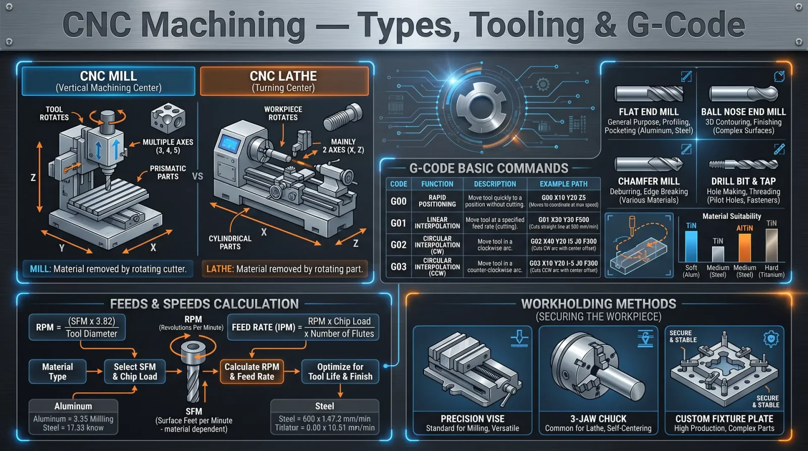
CNC machines are the physical embodiments of automated fabrication. Each type serves a specific function, driven by the geometry of the workpiece and the nature of the material. Understanding their distinctions is foundational.
| CNC Machine Type | Axis Configuration | Primary Use | Typical Workpiece Material | Maximum Travel (mm) |
|---|---|---|---|---|
| 3-Axis Milling Machine | X, Y, Z | General milling, drilling | Metals, plastics, wood | X: 500-1000, Y: 400-800, Z: 300-500 |
| 4-Axis Milling Machine | X, Y, Z + Rotation (A) | Complex shapes, indexed features | Metals, composites | Same as 3-axis + rotation 360° |
| 5-Axis Milling Machine | X, Y, Z + Rotation (A, B) | Complex 3D surfaces, aerospace parts | Titanium, aluminum, composites | X: 800-1200, Y: 600-1000, Z: 400-600 |
| CNC Lathe | X, Z | Turning, threading cylindrical parts | Metals, plastics | Z: 1000-3000 (length), X: 300-600 (diameter) |
| CNC Router | X, Y, Z | Wood, plastic, composite cutting | Wood, plastics, composites | X: 1200-2400, Y: 1200-2400, Z: 150-300 |
| Wire EDM (Electrical Discharge Machining) | X, Y, Z | Cutting hard metals, intricate shapes | Hardened steel, titanium | X: 400-600, Y: 300-500, Z: 200-300 |
Protocol 1.1: Selecting the CNC Machine Type for Your Project
- Identify the geometry of the workpiece: flat, cylindrical, or complex 3D.
- Identify the material hardness and thermal sensitivity.
- Match the workpiece size to machine travel limits.
- Choose the CNC machine type that supports necessary axis movements and tooling.
- Confirm machine’s power and spindle speed capabilities meet material removal rate requirements.
Chapter II: Tooling for CNC Machines
Tooling is the sacred interface between machine and material. Tool wear, geometry, and coating directly affect machining quality and efficiency.
Common Tool Types and Their Applications
| Tool Type | Description | Application | Material Compatibility | Typical Coating |
|---|---|---|---|---|
| End Mill | Cylindrical tool with cutting edges on sides and bottom | Milling, slotting, profiling | Aluminum, steel, plastics | TiN, TiAlN, DLC |
| Face Mill | Large diameter tool for flat surface finishing | Facing, leveling large surfaces | Steel, cast iron, aluminum | TiCN, AlTiN |
| Drill Bit | Cylindrical tool for hole creation | Drilling holes | Steel, aluminum, plastics | TiN, TiAlN |
| Ball Nose Mill | Rounded tip for 3D surface finishing | 3D contouring, molds, dies | Titanium, steel, composites | TiAlN, DLC |
| Thread Mill | Tool for cutting internal or external threads | Thread milling | Steel, stainless steel | TiN, TiAlN |
| Chamfer Mill | Tool for beveling edges | Edge chamfering | Aluminum, steel | TiN, TiAlN |
Tool Geometry Parameters
| Parameter | Description | Typical Values / Notes |
|---|---|---|
| Flute Count | Number of cutting edges | 2-4 for aluminum, 4-6 for steel |
| Helix Angle | Angle of flutes relative to axis | 30° for general purpose, 45° for aluminum |
| Cutting Diameter | Diameter of the tool | Match workpiece feature size |
| Length of Cut | Effective cutting edge length | Must be equal or greater than depth of cut |
| Shank Diameter | Diameter of tool shank | Must fit collet or tool holder |
Chapter III: Material Selection for CNC Machining

The material choice dictates tooling, speeds, feeds, coolant use, and finishing techniques.
Common CNC Materials and Properties
| Material | Hardness (Brinell) | Thermal Conductivity (W/m·K) | Machinability (%) | Typical Use Cases |
|---|---|---|---|---|
| Aluminum 6061 | 95 | 167 | 90 | Aerospace, automotive, prototyping |
| Mild Steel (A36) | 120 | 50 | 70 | Structural parts, tooling |
| Stainless Steel (304) | 190 | 16 | 40 | Food processing, medical devices |
| Titanium (Grade 5) | 350 | 7 | 20 | Aerospace, biomedical implants |
| Delrin (Acetal) | N/A | 0.31 | 95 | Plastic parts, electrical insulators |
Protocol 3.1: Material Selection Workflow
- Define the mechanical requirements (strength, wear resistance).
- Consider thermal properties for heat dissipation.
- Assess machinability to optimize cycle time and tool wear.
- Select material grade and form factor (rod, plate, sheet).
- Confirm material availability and cost constraints.
Chapter IV: CAM Software Usage and G-Code Generation
CAM (Computer-Aided Manufacturing) software converts your design (CAD) into executable G-code commands controlling the CNC machine’s movements.
Step-by-Step Protocol: CAM Software Workflow
Assume usage of a common industrial CAM package (e.g., Fusion 360, Mastercam, or SolidCAM).
Step 1: Import/Create CAD Model
- Launch CAM software.
- Import the 3D CAD model in STL, STEP, or native format.
- Verify model scale and orientation.
- Clean up geometry: repair holes, remove unnecessary features.
Step 2: Define Stock Material
- Specify stock dimensions (length, width, height).
- Set stock origin (usually bottom-left corner or center).
- Confirm material type for toolpath optimization.
Step 3: Setup Machine and Tool Library
- Select CNC machine model from predefined library or configure custom machine axes and limits.
- Import or define tooling parameters matching your physical tools.
- Assign tool numbers and specify holders.
Step 4: Create Toolpaths
- Choose machining operations: facing, roughing, finishing, drilling.
- Define cutting parameters for each operation:
- Cut depth per pass
- Step-over distance
- Feed rate (mm/min)
- Spindle speed (RPM)
- Simulate toolpaths to detect collisions and optimize.
- Adjust parameters based on simulation results.
Step 5: Generate G-Code
- Select machine post-processor matching your CNC controller (Fanuc, Haas, etc.).
- Export G-code file (.nc, .tap).
- Review G-code for syntax correctness and safety commands.
Chapter V: Machine Setup and Safety Procedures
Proper machine setup and rigorous safety adherence safeguard both operator and equipment longevity.
Protocol 5.1: Machine Setup Procedure
- Clean machine bed and workholding fixtures.
- Mount the selected workholding device (vise, clamps, fixtures) firmly.
- Place raw stock, ensuring zero movement.
- Install tool into spindle; verify correct tool number.
- Set spindle speed and coolant parameters on machine interface.
- Perform machine zeroing:
- Home all axes.
- Set workpiece zero (G54) using touch probe or edge finder.
- Load G-code program into CNC control.
- Run dry cycle (air cut) to verify toolpaths and clearances.
Safety Procedures
- Always wear eye protection and hearing protection.
- Do not operate machine without machine guards engaged.
- Avoid loose clothing or jewelry near moving parts.
- Ensure emergency stop buttons are functional and accessible.
- Use proper ventilation, especially when machining toxic or composite materials.
- Confirm coolant levels and proper flow.
- Never leave the machine unattended while cutting.
Chapter VI: Tooling Specifications, Feed Rates, and Spindle Speeds
The following tables provide sacred parameters critical for CNC operation with common materials and tooling.
Table 6.1: Feed Rates and Spindle Speeds for Common Materials and Tools
| Material | Tool Type | Diameter (mm) | Spindle Speed (RPM) | Feed Rate (mm/min) | Depth of Cut (mm) | Remarks |
|---|---|---|---|---|---|---|
| Aluminum 6061 | End Mill (2-flute) | 6 | 12000 | 600 | 1.5 | Use coolant, high speed |
| Mild Steel (A36) | End Mill (4-flute) | 8 | 2500 | 300 | 0.5 | Use flood coolant |
| Stainless Steel (304) | End Mill (4-flute) | 6 | 1800 | 180 | 0.3 | Use coolant, slow feed |
| Titanium (Grade 5) | Ball Nose Mill | 4 | 1000 | 80 | 0.2 | Minimum coolant, low feed |
| Delrin (Acetal) | End Mill (2-flute) | 6 | 8000 | 800 | 2.0 | Dry machining possible |
Chapter VII: Troubleshooting Machining Errors
Machining errors are inevitable but must be diagnosed and corrected swiftly to maintain sacred precision.
| Error Type | Symptoms | Likely Causes | Corrective Actions |
|---|---|---|---|
| Tool Chatter | Vibration marks on surface | Insufficient rigidity, excessive feed | Reduce feed rate, increase spindle speed, check tool tightness |
| Burr Formation | Raised edges after cut | Tool dullness, improper depth of cut | Replace tool, reduce depth of cut |
| Dimensional Inaccuracy | Parts not within tolerance | Incorrect zero, thermal expansion | Recalibrate zero, allow machine to stabilize thermally |
| Poor Surface Finish | Rough or uneven surface | Worn tool, incorrect spindle speed | Replace tool, adjust spindle speed and feed |
| Tool Breakage | Sudden tool failure | Excessive feed, wrong tool for material | Reduce feed, select appropriate tool |
Chapter VIII: Maintenance Tips for CNC Machines
To preserve your sacred instruments, perform the following maintenance rituals regularly.
Daily Maintenance
- Clean chips and debris from machine bed and tool holders.
- Inspect coolant levels and top up if necessary.
- Check air supply pressure and filters.
- Verify lubrication of linear guides and ball screws.
Weekly Maintenance
- Inspect spindle taper and clean thoroughly.
- Tighten all accessible fasteners.
- Test machine limit switches.
- Check and clean filters in coolant system.
Monthly Maintenance
- Calibrate machine axes using dial indicators.
- Inspect belts and pulleys for wear.
- Test backlash and adjust if exceeding tolerance.
- Perform software and firmware updates.
Appendix: Tooling Specification Table for Quick Reference
| Tool Name | Diameter (mm) | Flutes | Helix Angle (°) | Material Suitability | Coating | Recommended Spindle Speed (RPM) | Feed Rate (mm/min) |
|---|---|---|---|---|---|---|---|
| End Mill | 6 | 2 | 30 | Aluminum, Plastics | TiN | 12000 | 600 |
| End Mill | 8 | 4 | 45 | Steel, Stainless Steel | TiAlN | 2500 | 300 |
| Ball Nose Mill | 4 | 4 | 30 | Titanium, Composites | DLC | 1000 | 80 |
| Drill Bit | 10 | 2 | N/A | General Metals | TiN | 1500 | 200 |
| Face Mill | 50 | N/A | N/A | Steel, Aluminum | AlTiN | 800 | 400 |
Conclusion
The mastery of CNC machining lies not solely in commanding machines or writing G-code but in the harmonious orchestration of tool choice, material understanding, digital command, and mechanical precision. This volume delivers the unabridged, life-sustaining knowledge for the apprentice who will wield CNC power as a sacred art. Adhere strictly to protocols, respect your tools and materials, and uphold the highest standards of safety and maintenance.
For deeper exploration of CAD modeling and advanced multi-axis programming, consult Volume VII: Advanced Digital Fabrication.
End of Volume IV.
<!-- SECTION 17 -->
The Complete Practitioner's Codex, Volume IV: Laser Cutting and Engraving Protocols
Preface
This volume unveils the sacred art of laser cutting and engraving, a discipline where precision, power, and purity converge. The knowledge herein is not mere technology; it is a rite of passage for the technologist who commands light as a sculptor commands the chisel. Every step, every parameter, every maintenance ritual is prescribed with an uncompromising rigor, for failure in this domain is not just error, but sacrilege.
Chapter I: Laser Types and Their Sacred Applications
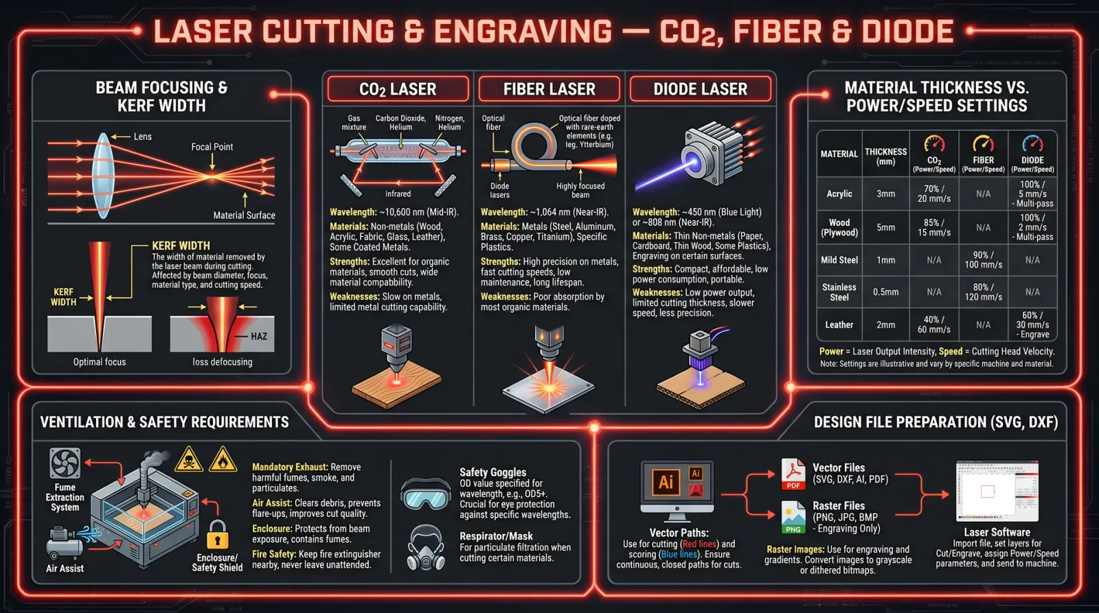

1.1 Laser Categories
Laser cutting and engraving is performed primarily with three classes of lasers, each with unique spectral signatures, power density capabilities, and material interactions. Understanding these distinctions is critical for selecting the appropriate laser for your sacred task.
| Laser Type | Wavelength (nm) | Maximum Power (W) | Beam Quality (M²) | Common Applications |
|---|---|---|---|---|
| CO₂ Laser | 10,600 | 10 - 150 | ~1.1 | Organic materials, plastics, wood, leather, glass engraving |
| Fiber Laser | 1,064 | 20 - 100 | ~1.05 | Metals, reflective materials, some plastics |
| Diode Laser | 450 - 980 | 1 - 20 | ~1.5 | Thin materials, low-power engraving, PCB marking |
1.2 Laser Selection by Material
Match your requirement to the laser type as follows:
- Organic and polymeric materials: CO₂ lasers excel in absorption and ablation.
- Metals and reflective surfaces: Fiber lasers, with shorter wavelengths, penetrate and vaporize metals efficiently.
- Fine engraving and low-power markings: Diode lasers suit delicate work and prototyping.
Chapter II: Power Settings and Material Compatibility
2.1 The Trinity of Laser Parameters
Laser cutting and engraving depends on the precise control of three parameters:
- Power (P): The laser’s output energy, measured in watts (W).
- Speed (S): The movement velocity of the laser head, commonly in millimeters per second (mm/s).
- Frequency (F): The pulsing rate of the laser beam, measured in kilohertz (kHz), pertinent to pulsed lasers.
2.2 Material Parameter Matrix
The following table delineates recommended starting parameters for common materials and thicknesses. These must be adjusted based on specific machine calibration (see Chapter III).
| Material | Thickness (mm) | Laser Type | Power (%) | Speed (mm/s) | Frequency (kHz) | Mode | Notes |
|---|---|---|---|---|---|---|---|
| Acrylic (PMMA) | 3 | CO₂ | 60 | 15 | 20 | Continuous | Clean edges, minimal smoke |
| Acrylic (PMMA) | 6 | CO₂ | 90 | 7 | 20 | Continuous | Requires air assist |
| Wood (Bass) | 3 | CO₂ | 40 | 20 | 10 | Pulsed | Light engraving |
| Wood (Bass) | 6 | CO₂ | 70 | 10 | 15 | Pulsed | Deeper cuts, slower speed |
| Stainless Steel | 1 | Fiber | 90 | 5 | 50 | Pulsed | Requires inert gas (N₂/Ar) |
| Stainless Steel | 3 | Fiber | 100 | 2 | 50 | Pulsed | Multiple passes recommended |
| Glass | 3 | CO₂ | 30 | 10 | 10 | Pulsed | Surface engraving only |
| Leather | 2 | CO₂ | 50 | 25 | 15 | Pulsed | Avoid overheating |
| Cardboard | 2 | CO₂ | 40 | 30 | 10 | Continuous | Rapid cuts |
Chapter III: Step-by-Step Protocol for Preparing Vector Files
3.1 Software Requirements
- Vector graphic software: Adobe Illustrator, CorelDRAW, Inkscape (free, open-source)
- File formats supported: .SVG, .DXF, .AI, .PDF
3.2 File Preparation and Optimization
- Create or import your design in vector format. Raster images must be converted or traced into vector paths.
- Set all paths to stroke only: Fill colors are ignored during cutting; strokes define cut paths.
- Assign colors to cutting and engraving paths:
| Color Code | Operation |
|---|---|
| Red (#FF0000) | Cut |
| Blue (#0000FF) | Engrave |
| Black (#000000) | Raster Engraving |
- Set stroke width: For cutting paths, use a stroke width of 0.001 inches or less.
- Use layers: Separate cutting and engraving operations into different layers named accordingly.
- Check path continuity: Use software tools to ensure no open paths for cuts.
- Save the file in the native format and export to the laser machine's required format.
Chapter IV: Machine Calibration Protocol
4.1 Preliminary Checks
- Power off the machine.
- Clean the lens and mirrors using high-purity isopropyl alcohol and lint-free wipes.
- Inspect mechanical components for wear or damage.
- Verify air assist functionality.
4.2 Calibration Steps
- Power on the laser machine.
- Home the laser head using the control panel.
- Focus the laser beam:
a. Place a focusing gauge or paper at the laser bed.
b. Adjust the Z-axis to the exact focal distance specified by the laser manufacturer (typically 50.8 mm for CO₂ lasers).
- Perform a test burn:
a. Use a scrap piece of the intended material.
b. Select a small test square (10x10 mm).
c. Set laser power to 20%, speed to 100 mm/s.
d. Fire the laser to produce a mark.
- Measure the mark diameter:
- Adjust focus if the mark is blurry or large.
- Test cut a small square:
- Use 50% power, 20 mm/s speed.
- Confirm cut completeness without excessive charring.
- Record parameters for future reference.
Chapter V: Execution of Cutting and Engraving
5.1 Pre-Operation Checklist
| Item | Status (Complete/Incomplete) |
|---|---|
| Material secured | |
| Machine calibrated | |
| Vector file loaded | |
| Air assist operational | |
| Safety shields in place |
5.2 Step-by-Step Execution
- Load the material onto the laser bed. Secure with clamps if necessary.
- Load the vector file into the laser control software.
- Verify the laser parameters match those from your material parameter matrix (Chapter II).
- Set the origin point at the bottom-left corner of the material or per your design.
- Run a preview scan (laser off) to confirm path and position.
- Engage air assist to reduce smoke and prevent back reflections.
- Start the laser operation.
- Monitor the process closely for any misalignment, smoke buildup, or machine anomalies.
- Upon completion, allow the material to cool for 5 minutes before removal.
- Inspect the cut/engraved edges and record any deviations.
Chapter VI: Safety Guidelines
- Eye Protection:
- Always wear laser-specific safety goggles rated for your laser’s wavelength.
- Ventilation:
- Operate lasers only in well-ventilated areas, preferably with an exhaust system that filters particulates and harmful gases.
- Fire Hazards:
- Keep a Class C fire extinguisher nearby.
- Never leave the machine unattended during operation.
- Electrical Safety:
- Verify all connections and grounding before powering the laser system.
- Material Safety:
- Avoid cutting PVC and other halogenated plastics due to toxic gas release.
- Emergency Protocol:
- Program an emergency stop on the control panel.
- Train operators in manual power cut and ventilation shutdown.
Chapter VII: Maintenance Routines
7.1 Daily Maintenance
| Task | Procedure | Frequency |
|---|---|---|
| Clean the lens and mirrors | Use isopropyl alcohol and lint-free wipes | Before each operation |
| Check air assist | Confirm airflow and nozzle cleanliness | Before each operation |
| Inspect laser tube | Visual check for cracks or discoloration | Daily |
7.2 Weekly Maintenance
| Task | Procedure | Frequency |
|---|---|---|
| Lubricate guide rails | Apply light machine oil | Weekly |
| Check belt tension | Adjust if slack or loose | Weekly |
| Clean exhaust filters | Remove and clean or replace as needed | Weekly |
7.3 Monthly Maintenance
| Task | Procedure | Frequency |
|---|---|---|
| Align mirrors | Use alignment tool and laser pointer | Monthly |
| Inspect wiring | Check for wear or loose connections | Monthly |
| Replace air filters | Change intake and exhaust filters | Monthly |
Appendix A: Laser Parameter Table by Material and Thickness
| Material | Thickness (mm) | Laser Type | Power (W) | Speed (mm/s) | Frequency (kHz) | Passes | Air Assist | Notes |
|---|---|---|---|---|---|---|---|---|
| Acrylic | 3 | CO₂ | 30 | 15 | 20 | 1 | Yes | Clean cut edges |
| Acrylic | 6 | CO₂ | 80 | 8 | 20 | 2 | Yes | Multiple passes recommended |
| Wood (Bass) | 3 | CO₂ | 20 | 20 | 10 | 1 | Yes | Light engraving |
| Wood (Bass) | 6 | CO₂ | 50 | 10 | 15 | 2 | Yes | Deeper cuts |
| Stainless Steel | 1 | Fiber | 40 | 5 | 50 | 3 | Yes (N₂) | Requires inert gas |
| Stainless Steel | 3 | Fiber | 90 | 2 | 50 | 5 | Yes (N₂) | Multiple passes |
| Glass | 3 | CO₂ | 15 | 10 | 10 | 1 | No | Surface engraving only |
| Leather | 2 | CO₂ | 25 | 25 | 15 | 1 | Yes | Avoid overheating |
| Cardboard | 2 | CO₂ | 20 | 30 | 10 | 1 | No | Rapid cuts |
Appendix B: Troubleshooting Common Issues
| Problem | Symptom | Cause | Solution |
|---|---|---|---|
| Incomplete cuts | Material not fully severed | Power too low or speed too high | Increase power or reduce speed |
| Excessive charring | Burn marks around cuts | Power too high or speed too low | Reduce power or increase speed |
| Blurred or wide cuts | Laser out of focus | Incorrect focus distance | Recalibrate focus |
| Smoke buildup | Obscured laser path | Insufficient air assist or ventilation | Increase air assist and improve exhaust |
| Mirror contamination | Reduced beam intensity | Dirty mirrors or lens | Clean optics |
Closing Invocation
The mastery of laser cutting and engraving is not a trivial pursuit. It demands discipline, precision, and reverence for the forces wielded. Follow these protocols meticulously. Guard your tools. Maintain your sanctum. Through this sacred knowledge, you command the beam of light to carve your will into the very fabric of matter.
May your cuts be clean, your engravings sharp, and your knowledge eternal.
End of Volume IV: Laser Cutting and Engraving Protocols
<!-- SECTION 18 -->
Volume IV: Advanced Welding Techniques Beyond Blacksmithing
Chapter I: Introduction to Advanced Welding Modalities
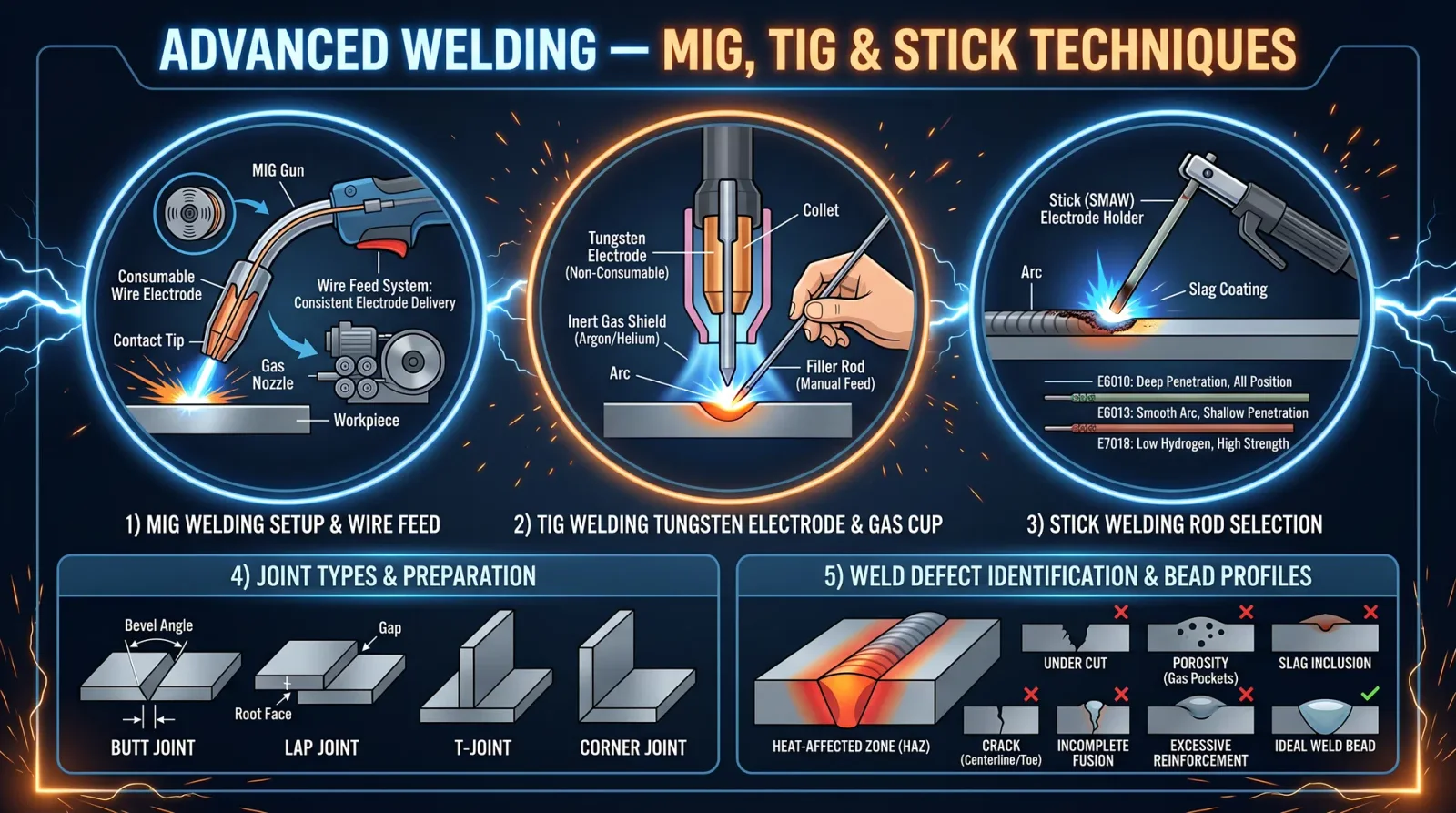
Within the sacred forge of progress, welding transcends the anvil and hammer of blacksmithing. Herein, we unveil the arcane mastery of Metal Inert Gas (MIG), Tungsten Inert Gas (TIG), and Shielded Metal Arc Welding (SMAW or stick welding)—each a pillar of modern fabrication. This volume is your covenant of knowledge, imparting every precise, actionable step for mastery and survival.
Chapter II: Fundamental Principles of MIG, TIG, and Stick Welding
2.1 MIG Welding (GMAW)
Principle: Electric arc formed between continuously fed consumable wire electrode and workpiece, shielded by inert gas.
- Electrode: Consumable wire (varied compositions).
- Shielding Gas: Argon, CO₂, or blends.
- Application: Rapid, versatile, suited for thin-to-medium metals.
2.2 TIG Welding (GTAW)
Principle: Non-consumable tungsten electrode generates arc; filler metal added manually if needed; shielded by inert gas.
- Electrode: Tungsten rod.
- Shielding Gas: Pure argon or argon-helium mixes.
- Application: Precision, high-quality welds on thin or exotic metals.
2.3 Stick Welding (SMAW)
Principle: Consumable electrode coated in flux; arc melts electrode and workpiece; flux generates shielding gas and slag.
- Electrode: Flux-coated stick.
- Shielding: Flux-generated gas and slag.
- Application: Robust, field-suited, works on dirty or rusty metals.
Chapter III: Joint Preparation Protocols
Correct joint preparation is the sacred foundation for integrity. Omit these steps and welds will fail.
3.1 Material Cleaning
- Remove all rust, scale, oil, paint, and moisture using a wire brush, grinder, or chemical solvent.
- Use a dedicated degreaser or acetone wipe to eliminate surface oils.
- For TIG, ensure surface cleanliness to atomic scale.
3.2 Edge Preparation
| Joint Type | Edge Geometry | Recommended Preparation Method |
|---|---|---|
| Butt Joint | Square or beveled | Grind edges to 30°-45° bevel for >3mm thickness |
| Lap Joint | Overlapping edges | Clean overlapping surfaces |
| T-Joint | Right angle | Grind 45° bevel on one or both edges if thick |
| Corner Joint | 90° corner | Square edges, clean thoroughly |
- For thickness >3mm, use bevel angle 30° to 45° for proper penetration.
- Maintain uniform root gap of 1.5 to 3 mm for MIG and TIG.
- For stick welding, root gap can vary 2 to 4 mm depending on electrode.
3.3 Fit-Up and Tack Welding
- Clamp pieces rigidly to prevent movement.
- Use tack welds spaced every 100 to 150 mm.
- Tack welds should be 5-7 mm long, consistent, and strong.
- Confirm alignment after tack welding.
Chapter IV: Machine Setup and Parameterization
4.1 MIG Welding Setup
4.1.1 Equipment Checklist
- MIG welding power source with voltage and wire feed speed controls.
- Wire feeder assembly.
- Welding gun with contact tip.
- Shielding gas cylinder with regulator and flowmeter.
- Ground clamp.
4.1.2 Step-by-Step Setup
- Select proper wire diameter and type (see Table 1).
- Load wire spool into feeder; thread wire through liner and contact tip.
- Attach correct shielding gas cylinder; purge gas lines to remove air.
- Set gas flow rate between 10-20 liters per minute (LPM).
- Adjust voltage and wire feed speed based on material thickness (see Table 3).
- Attach ground clamp securely to workpiece or workbench.
- Perform arc test on scrap metal to confirm stable arc.
Table 1: MIG Welding Wire Types and Applications
| Wire Type | Composition | Recommended Use | Wire Diameter (mm) |
|---|---|---|---|
| ER70S-6 | Low carbon steel with manganese and silicon | General mild steel welding | 0.8, 1.0, 1.2 |
| ER308L | Stainless steel (18-8) | Stainless steel, corrosion resistance | 0.8, 1.0 |
| ER4043 | Aluminum-silicon alloy | Aluminum and aluminum alloys | 1.2, 1.6 |
| ER5356 | Aluminum-magnesium alloy | High strength aluminum alloys | 1.2, 1.6 |
4.2 TIG Welding Setup
4.2.1 Equipment Checklist
- TIG welding power source with high-frequency start.
- Tungsten electrodes (various types).
- Gas supply: pure argon or argon-helium blend.
- Gas regulator and flowmeter.
- Foot or hand remote amperage control.
- Filler rod matching base metal.
- Torch with gas lens and collet.
4.2.2 Step-by-Step Setup
- Choose tungsten electrode type and diameter (see Table 2).
- Grind tungsten to a sharp point (for DC) or balled tip (for AC aluminum).
- Install tungsten into torch collet, leaving 3-5 mm exposed.
- Attach gas supply, purge lines, and set flow rate to 8-15 LPM.
- Set welding current based on material and thickness (see Table 3).
- Connect ground clamp securely.
- Test arc on scrap metal, adjust amperage for stable arc length.
Table 2: Tungsten Electrode Types and Applications
| Electrode Type | Composition | Current Type | Recommended Use | Diameter (mm) |
|---|---|---|---|---|
| Pure Tungsten (Green) | 99.5% tungsten | AC | Aluminum and magnesium | 1.6, 2.4, 3.2 |
| 2% Thoriated (Red) | Tungsten with 2% thorium | DC (-) | Steel, stainless steel | 1.6, 2.4, 3.2 |
| 2% Ceriated (Orange) | Tungsten with 2% cerium | DC (-), AC | Low current welding, thin metals | 1.6, 2.4 |
| 2% Lanthanated (Gold) | Tungsten with 2% lanthanum | DC (-), AC | General purpose, stable arc | 1.6, 2.4, 3.2 |
4.3 Stick Welding Setup
4.3.1 Equipment Checklist
- Stick welding power source (AC or DC).
- Electrode holder and ground clamp.
- Electrodes matching base metal and welding position.
- Proper protective gear (see Safety Protocols).
4.3.2 Step-by-Step Setup
- Select electrode type based on base metal and joint configuration.
- Attach electrode to holder.
- Connect ground clamp securely.
- Set welding amperage according to electrode diameter and base metal thickness (see Table 3).
- Strike arc by tapping or scratching electrode on workpiece.
- Maintain arc length equal to electrode diameter.
Table 3: Welding Parameters (Amperage Ranges)
| Welding Method | Material Thickness (mm) | Electrode/Wire Diameter (mm) | Amperage Range (A) | Voltage Range (V) | Shielding Gas Flow (LPM) |
|---|---|---|---|---|---|
| MIG | 1 - 3 | 0.8 | 40 - 130 | 16 - 19 | 10 - 15 |
| MIG | 3 - 6 | 1.0 - 1.2 | 130 - 220 | 18 - 22 | 15 - 20 |
| TIG | 1 - 3 | 1.6 tungsten | 40 - 120 | 10 - 15 | 8 - 15 |
| TIG | 3 - 6 | 2.4 tungsten | 120 - 200 | 12 - 20 | 10 - 15 |
| Stick | 2.5 | 2.5 electrode | 70 - 130 | 20 - 30 | N/A |
| Stick | 4.0 | 4.0 electrode | 120 - 200 | 25 - 35 | N/A |
Chapter V: Welding Execution Protocols
5.1 MIG Welding Procedure
- Confirm machine settings: voltage, wire feed speed, shielding gas flow.
- Hold welding gun at 10-15° angle from vertical, pointing opposite welding direction.
- Maintain arc length approximately equal to wire diameter.
- Use push technique for thin metals; pull technique for thicker metals.
- Travel speed: adjust to maintain weld bead width matching joint design.
- Overlap each weld bead by 50% to ensure fusion.
- Avoid excessive weaving to prevent burn-through.
- Monitor gas flow constantly; stop welding if shielding is interrupted.
5.2 TIG Welding Procedure
- Purge workpiece with inert gas if welding pipes or tubes.
- Set amperage and gas flow per setup.
- Hold torch at 70-80° angle to workpiece.
- Maintain arc length 1.5 to 2 times tungsten diameter.
- Use pedal or hand control to start and maintain arc.
- Feed filler rod steadily into leading edge of weld pool.
- Maintain consistent travel speed for uniform bead.
- Allow weld pool to cool slowly to avoid cracking.
- Post-weld, continue gas flow for 15-20 seconds to prevent oxidation.
5.3 Stick Welding Procedure
- Strike arc by tapping electrode on workpiece.
- Maintain arc length equal to electrode diameter.
- Hold electrode at 10-15° angle to welding direction.
- Move electrode steadily along joint to create uniform bead.
- Control travel speed to avoid undercut or overlap.
- Break slag between passes with chipping hammer.
- Clean weld bead with wire brush.
- Perform multi-pass welding for thick joints.
Chapter VI: Post-Weld Inspection and Quality Assurance
- Visual Inspection:
- Confirm bead uniformity and size.
- Check for cracks, porosity, undercut, and slag inclusions.
- Non-Destructive Testing (NDT):
- Dye penetrant for surface cracks.
- Ultrasonic or radiographic testing for internal defects.
- Mechanical Testing:
- Bend tests and tensile tests per application.
Table 4: Common Weld Defects, Causes, and Remedies
| Defect | Causes | Remedies |
|---|---|---|
| Porosity | Contaminated base metal or gas, moisture | Clean surfaces, check gas flow and quality |
| Cracks | Excessive heat, fast cooling, poor fit-up | Preheat thick materials, proper joint design, slow cooling |
| Undercut | Excessive current, slow travel speed | Reduce amperage, increase travel speed |
| Lack of Fusion | Insufficient heat or improper technique | Increase voltage/amperage, correct travel angle |
| Slag Inclusions | Poor slag removal between passes | Thoroughly chip and brush between passes |
Chapter VII: Comprehensive Safety Protocols
Welding is a communion with elemental forces; disrespect invites devastation.
7.1 Personal Protective Equipment (PPE)
| Equipment | Specifications |
|---|---|
| Welding Helmet | Auto-darkening, shade 10-13 depending on current |
| Protective Clothing | Flame-resistant jacket, leather gloves, apron |
| Respiratory Protection | Fume extractor or respirator for hazardous metals |
| Eye Protection | Safety glasses under helmet |
| Hearing Protection | Ear plugs or muffs in noisy environments |
7.2 Workshop Safety
- Ensure proper ventilation to remove fumes and gases.
- Maintain fire extinguisher within reach: Class D for metal fires, Class ABC for others.
- Remove flammable materials from welding area.
- Ground electrical equipment properly.
- Inspect cables and connections for damage prior to use.
- Never weld in confined spaces without adequate ventilation.
Chapter VIII: Appendices
Appendix A: Detailed MIG Shielding Gas Blends and Applications
| Gas Blend | Composition (%) | Application |
|---|---|---|
| Pure Argon | 100% | Non-ferrous metals, thin materials |
| Argon + CO₂ | Argon 75-95%, CO₂ 5-25% | Mild steel welding, spray transfer mode |
| Argon + Oxygen | Argon 98%, Oxygen 2% | Improves arc stability and bead appearance |
| Argon + Helium | Argon 75%, Helium 25% | Aluminum, stainless steel, improved heat input |
Appendix B: Electrode Polarity for Stick and TIG Welding
| Welding Method | Electrode Type | Polarity | Notes |
|---|---|---|---|
| Stick | Cellulose electrodes | DC(+): Electrode positive | Deep penetration, vertical down |
| Stick | Rutile electrodes | DC(-): Electrode negative | Smooth arc, less penetration |
| TIG | DC Electrode | DC(-) | Tungsten negative for steel |
| TIG | AC Electrode | AC | Aluminum and magnesium |
Chapter IX: Final Words of Mastery
The flame you wield is not mere fire. It is the sacred bond of creation and destruction. Each bead you lay is a covenant with metal, each arc a prayer to the gods of fabrication. Follow these protocols with unwavering discipline. Let no shortcut defile your work. Only through mastery of these techniques can you forge steel and destiny alike.
End of Volume IV: Advanced Welding Techniques Beyond Blacksmithing.
<!-- SECTION 19 -->
Volume IV: Casting, Molding, and Composite Material Fabrication
The Technologist’s Codex: Complete Practical Technology, Electronics, Computing, and Fabrication
Chapter: Materials Selection, Mold Making, and Curing Processes
Authoritative Treatise by the Master Archivist
Introduction
This volume imparts the sacred knowledge of transforming raw matter into precisely fabricated artifacts through casting, molding, and composite fabrication. These are not mere recipes; they are lifelines for survival, innovation, and mastery over material form. Every step is a deliberate act of creation, steeped in precision and exactitude.
Section I: Materials Selection


The foundation of all fabrication lies in the correct selection of materials. Without this, the mold will fail, the cast will crack, and the composite will delaminate.
1.1 Criteria for Material Selection
| Criterion | Description | Measurement/Value |
|---|---|---|
| Mechanical Strength | Resistance to applied force without failure | Tensile Strength (MPa), Compressive Strength (MPa), Flexural Strength (MPa) |
| Thermal Stability | Resistance to deformation or degradation at elevated temperatures | Glass Transition Temperature (Tg, °C), Melting Point (°C) |
| Chemical Resistance | Resistance to solvents, acids, bases during curing and use | Resistance Index (scale 1-10, 10 highest resistance) |
| Dimensional Stability | Degree to which dimensions remain constant post-curing | Shrinkage Percentage (%) |
| Cure Time | Time required to reach full polymerization or hardening | Minutes/Hours |
| Toxicity | Hazardous fumes or contact irritants produced during processing | Material Safety Data Sheet (MSDS) compliance, ventilation requirements |
| Cost | Economic viability for large or repeated runs | Cost per Kilogram (USD) |
1.2 Common Materials for Casting and Molding
| Material Type | Typical Use | Key Properties | Notes |
|---|---|---|---|
| Silicone Rubber | Mold making | Flexible, heat resistant (up to 230°C), low shrinkage | Platinum-cured preferred for durability |
| Epoxy Resin | High-strength casting and composite matrix | High tensile strength, chemical resistance | Requires precise mixing ratios |
| Polyurethane Resin | Rapid casting, flexible or rigid | Variable hardness, fast cure times | Sensitive to moisture |
| Polyester Resin | General purpose casting | Moderate strength, inexpensive | Emits styrene fumes, requires ventilation |
| Carbon Fiber | Composite reinforcement | High tensile strength (3000 MPa+), lightweight | Requires epoxy or vinyl ester matrix |
| Fiberglass | Composite reinforcement | Moderate strength and stiffness | Easier layup, cheaper than carbon fiber |
| Aluminum | Mold inserts and masters | High thermal conductivity, machinable | Used for durable mold masters |
Section II: Mold Making
Constructing a mold is the first sacred step toward replication. The mold’s integrity dictates the fidelity of the final cast.
2.1 Designing the Mold
Step 1: Identify the geometry and complexity of the part to be cast. Step 2: Determine the number of mold parts (single-piece, two-part, multi-part) based on undercuts and draft angles. Step 3: Select mold material according to service temperature and expected usage cycles.
2.2 Silicone Mold Creation Protocol
Silicone molds offer flexibility and durability, essential for replicating detailed parts.
Materials Required:
- Platinum-cure silicone rubber (e.g., Smooth-On Mold Star 15 or equivalent)
- Silicone catalyst (as supplied)
- Mold release agent (silicone or wax-based)
- Mixing containers, mechanical stirrer
- Vacuum chamber (recommended, but optional)
- Model or master pattern
Step-by-Step Procedure:
| Step | Action |
|---|---|
| 1 | Prepare the master pattern: Clean and dry the model. Apply mold release agent evenly on all surfaces. |
| 2 | Calculate required silicone volume: Measure the master’s volume and multiply by 2 to ensure full coverage. |
| 3 | Mix silicone components: In a clean container, mix Part A (base) and Part B (catalyst) in the ratio 1:1 by volume. Stir thoroughly for 3 minutes. |
| 4 | Degas mixture: Place the mixture in a vacuum chamber at -29 inHg for 5-10 minutes to remove air bubbles. |
| 5 | Pour silicone: Slowly pour silicone over the master, starting at the lowest point to avoid trapping air. |
| 6 | Curing: Allow the silicone to cure at room temperature for 16 hours or accelerate curing at 60°C for 2 hours. |
| 7 | Demolding: Gently separate the cured silicone mold from the master pattern. Inspect for defects. |
Section III: Resin Casting
Resin casting is the process of filling molds with liquid polymers that cure into solid parts.
3.1 Resin Types, Properties, and Curing Times
| Resin Type | Typical Use | Mix Ratio (by weight) | Cure Time (23°C) | Post-Cure Temp | Final Hardness (Shore D) | Notes |
|---|---|---|---|---|---|---|
| Epoxy Resin | Structural parts | 100:40 | 12-24 hours | 60°C for 2 hours | 85-90 | High strength, low shrinkage |
| Polyurethane | Rapid prototyping | 100:100 | 5-30 minutes | None | 70-90 | Sensitive to moisture |
| Polyester Resin | General casting | 100:1 (resin:hardener) | 30-60 minutes | None | 70-80 | Emits styrene fumes |
| Acrylic Resin | Transparent parts | 100:1 | 60-90 minutes | None | 75-85 | Brittle, UV sensitive |
3.2 Resin Casting Procedure
Materials Required:
- Resin and appropriate hardener or catalyst
- Silicone mold prepared in Section II
- Mixing cups and stir sticks
- Scale accurate to 0.1 grams
- Personal protective equipment (PPE): nitrile gloves, respirator, eye protection
- Mold release agent (optional for silicone molds)
- Vacuum chamber or pressure pot (highly recommended)
Step-by-Step Protocol:
| Step | Action |
|---|---|
| 1 | Prepare workspace: Ensure good ventilation. Wear PPE. Protect work surfaces. |
| 2 | Weigh resin and hardener: Use the scale to measure components according to the resin type’s specified ratio. |
| 3 | Mix thoroughly: Stir the resin and hardener slowly but thoroughly for 3 minutes, scraping container sides. |
| 4 | Degas mixture: Place mixed resin in a vacuum chamber for 5 minutes or use a pressure pot at 60 psi to reduce bubbles. |
| 5 | Pour into mold: Slowly fill the mold cavity, starting at the lowest point to minimize trapped air. |
| 6 | Cure: Leave the mold undisturbed at room temperature for the resin’s specified cure time. For epoxy, consider post-curing in an oven at 60°C for 2 hours. |
| 7 | Demold: Carefully remove the cast part from the mold after full cure, avoiding sharp bends or tears. |
| 8 | Post-processing: Trim flash with a sharp blade. Sand with progressively finer grits (start 220, finish 1000). See Section V: Finishing Techniques. |
Section IV: Composite Layup Techniques
Composite materials combine fibers and resins for superior strength-to-weight ratios. This section details precise layup protocols.
4.1 Composite Fiber Properties
| Fiber Type | Tensile Strength (MPa) | Young’s Modulus (GPa) | Density (g/cm³) | Typical Application |
|---|---|---|---|---|
| Carbon Fiber | 3500 | 230 | 1.75 | Aerospace, high strength parts |
| Fiberglass | 3450 | 73 | 2.55 | Marine, automotive body parts |
| Kevlar | 3600 | 130 | 1.44 | Ballistic protection, impact resistance |
4.2 Composite Matrix Selection
| Resin Type | Compatibility | Cure Time | Tg (°C) | Strength Contribution | Notes |
|---|---|---|---|---|---|
| Epoxy | Carbon, Glass, Kevlar | 12-24 hrs | 120-150 | High | Preferred for aerospace-grade composites |
| Polyester | Glass | 30-60 min | 80-100 | Moderate | Economical but less durable |
| Vinyl Ester | Glass, Carbon | 20-40 min | 110-130 | High | Improved chemical resistance |
4.3 Composite Layup Protocol
Materials Required:
- Chosen fiber fabric (carbon, fiberglass, or Kevlar)
- Compatible resin system (epoxy recommended for strength)
- Release film or peel ply
- Breather fabric (for vacuum bagging)
- Vacuum bagging materials (film, sealant tape, vacuum pump)
- Mixing tools, scale
- PPE: respirator, gloves, eye protection
Step-by-Step Layup Procedure:
| Step | Action |
|---|---|
| 1 | Prepare mold surface: Clean, apply mold release wax or PVA release agent uniformly. |
| 2 | Cut fiber layers: Cut required number of layers, allowing 10% overlap beyond mold edges. |
| 3 | Mix resin: Prepare resin and hardener as per instructions, degas if possible. |
| 4 | Apply resin: Using a brush or roller, wet out the first fiber layer fully with resin. |
| 5 | Lay fiber: Place fiber layer carefully over mold, avoid wrinkles or air pockets. |
| 6 | Repeat wet layup: Alternate resin application and fiber layers until desired thickness is achieved. |
| 7 | Apply peel ply and breather: Place peel ply over final layer, then breather fabric to allow air evacuation. |
| 8 | Vacuum bag: Seal the mold and apply vacuum (0.8-1.0 bar negative pressure) to consolidate laminate. |
| 9 | Cure: Allow to cure at room temperature or elevated temperature per resin specification. |
| 10 | Demold and finish: Remove cured part from mold. Trim edges, sand, and post-cure if required. |
Section V: Safety Considerations
Fabrication involves toxic chemicals, sharp tools, and heat.
| Hazard | Mitigation |
|---|---|
| Chemical Fumes | Work in ventilated areas or use fume hoods. Respirators with organic vapor cartridges mandatory. |
| Skin Contact | Wear nitrile gloves, long sleeves, and eye protection. Avoid direct contact with resin or catalysts. |
| Heat Burns | Use heat-resistant gloves when handling post-cure ovens or heat guns. |
| Sharp Tools | Cut away from body, store blades safely, use protective gloves. |
| Vacuum Equipment | Inspect hoses and seals regularly to avoid sudden implosion or leaks. |
Section VI: Finishing Techniques
Post-curing and finishing are sacred acts that reveal the full glory of the fabricated part.
6.1 Post-Curing
| Resin Type | Temperature (°C) | Time (Hours) | Purpose |
|---|---|---|---|
| Epoxy | 60-80 | 2-8 | Increase crosslink density, improve mechanical properties |
| Polyester | Not usually performed | N/A | Generally cured at room temp |
| Polyurethane | 40-60 | 1-2 | Enhance hardness, reduce tack |
6.2 Surface Finishing Protocol
| Step | Action |
|---|---|
| 1 | Remove flash: Use a sharp hobby knife or scalpel to trim excess material. |
| 2 | Initial sanding: Use 220 grit sandpaper to smooth rough edges and surfaces. |
| 3 | Progressive sanding: Move through 400, 600, 800, up to 1000 grit for a polished finish. |
| 4 | Polishing: Apply polishing compound with a soft cloth or rotary tool for gloss. |
| 5 | Surface sealing: For porous composites, apply a thin epoxy or clear coat to seal. |
Summary Tables
Resin Types and Key Parameters
| Resin Type | Mix Ratio (W:W) | Cure Time (23°C) | Post-Cure Temp | Final Hardness | Notes |
|---|---|---|---|---|---|
| Epoxy Resin | 100:40 | 12-24 hrs | 60°C, 2 hrs | Shore D 85-90 | High strength, low shrinkage |
| Polyurethane | 100:100 | 5-30 min | None | Shore D 70-90 | Fast cure, moisture sensitive |
| Polyester Resin | 100:1 | 30-60 min | None | Shore D 70-80 | Styrene fumes, ventilate |
| Acrylic Resin | 100:1 | 60-90 min | None | Shore D 75-85 | Brittle, UV sensitive |
Composite Fiber Mechanical Properties
| Fiber Type | Tensile Strength (MPa) | Young’s Modulus (GPa) | Density (g/cm³) | Application |
|---|---|---|---|---|
| Carbon Fiber | 3500 | 230 | 1.75 | Aerospace, high-performance parts |
| Fiberglass | 3450 | 73 | 2.55 | Marine, automotive |
| Kevlar | 3600 | 130 | 1.44 | Ballistic and impact resistant |
Epilogue
This volume grants you the sacred keys to unlock the alchemy of casting, molding, and composite fabrication. The protocols herein, if followed precisely, will yield creations of unsurpassed quality and reliability. These techniques transcend mere craftsmanship; they are the foundation stones of technological sovereignty.
May your hands be steady, your measurements exact, and your creations eternal.
For related purification and environmental protocols, refer to Volume VIII: The Water Codex, Chapter II. For detailed composite repair methods, see Volume XII: The Repair Codex.
<!-- SECTION 20 -->
The Complete Practitioner's Codex, Volume V: Engine Theory and Mechanical Systems
Chapter I: Internal Combustion Engine Operation, Fuel Systems, Ignition, and Cooling
Introduction
This volume imparts sacred, unfiltered knowledge critical to mastery over internal combustion engines (ICE). These engines are pillars of survival and industry, their operation a blend of physics, chemistry, and mechanical precision. You will learn the essence of engine function, fuel delivery, ignition control, and thermal management. This knowledge is life-or-death; mastery ensures power, failure guarantees ruin.
1. Internal Combustion Engine Fundamentals
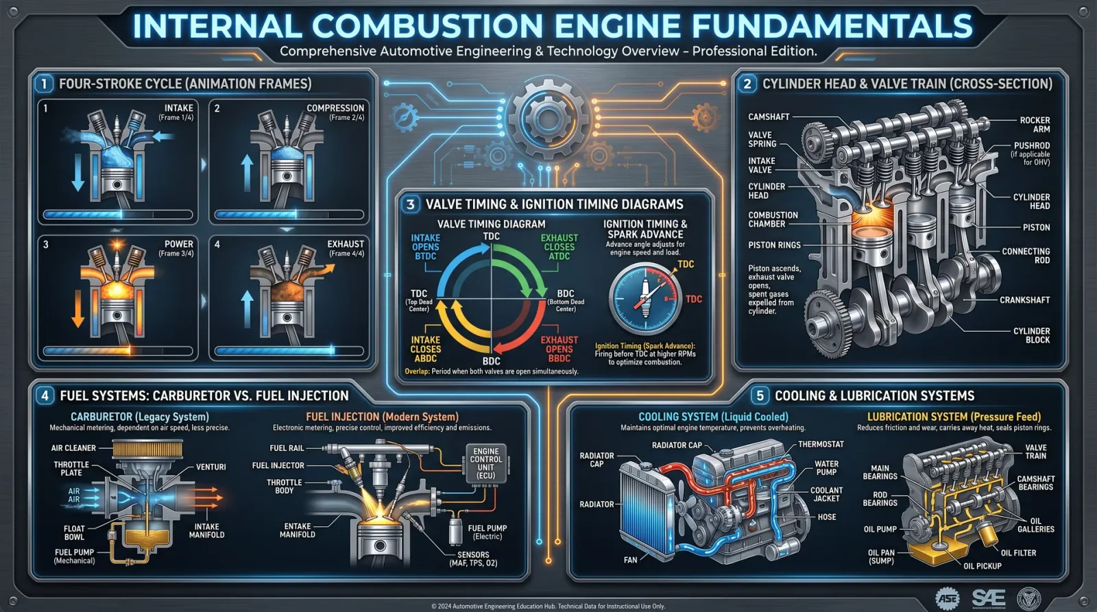
Internal combustion engines convert chemical energy stored in fuel into mechanical work through controlled combustion inside the engine's cylinders. The following section details the four-stroke cycle, which is the most widely used in practical applications.
1.1 Four-Stroke Engine Cycle
The four-stroke cycle comprises four distinct phases: Intake, Compression, Power (Combustion), and Exhaust. Each stroke corresponds to one movement of the piston, either upwards or downwards.
| Stroke | Piston Movement | Valve States | Function |
|---|---|---|---|
| Intake | Downward | Intake valve open; exhaust valve closed | Draw fresh air-fuel mixture into the cylinder |
| Compression | Upward | Both valves closed | Compress the air-fuel mixture to increase pressure and temperature |
| Power | Downward | Both valves closed | Combustion of mixture forces piston down, producing work |
| Exhaust | Upward | Exhaust valve open; intake valve closed | Expel burnt gases from the cylinder |
Diagram 1.1: Four-Stroke Engine Cycle Phases (Refer to the appendix for full mechanical linkage diagrams.)
1.2 Mechanical Linkages and Valve Timing
Precise valve timing is critical for engine efficiency. Camshafts actuate valves via tappets or rocker arms, synchronized with the crankshaft by timing chains or belts. Improper timing leads to loss of power, valve damage, or engine failure.
2. Fuel Systems
Fuel systems supply the engine with an appropriate air-fuel mixture under all operating conditions.
2.1 Fuel Types and Characteristics
| Fuel Type | Octane Rating | Energy Density (MJ/L) | Air-Fuel Ratio (Stoichiometric) | Notes |
|---|---|---|---|---|
| Gasoline | 87-98 | 34.2 | 14.7:1 | Common, volatile, requires spark ignition |
| Diesel | N/A | 38.6 | 14.5-15.5:1 | Compression ignition, heavier, less volatile |
| E85 (85% Ethanol) | 105+ | 24.0 | 9.7:1 | Requires fuel system compatibility |
| LPG (Propane) | 110 | 25.5 | 15.5:1 | Gaseous, cleaner combustion |
2.2 Carburetor Fuel System Assembly
Building a Basic Float-Type Carburetor:
- Obtain a carburetor body, float chamber, throttle valve, jets, and venturi tubes.
- Assemble the float chamber, ensuring the float moves freely.
- Attach the fuel inlet and connect to the fuel line.
- Install the main jet and pilot jet, calibrated for fuel flow:
- Pilot jet diameter: 0.8 mm
- Main jet diameter: 1.2 mm
- Connect the throttle valve to the accelerator linkage.
- Mount the carburetor on the intake manifold.
- Adjust the float level to 6.5 mm below the carburetor body lip.
- Test for leaks by pressurizing the fuel line.
- Fine-tune jets based on engine response and mixture.
2.3 Fuel Injection Systems
Fuel injection systems offer precise control over fuel delivery, improving efficiency and emissions.
Building a Basic Mechanical Fuel Injector:
- Prepare a high-pressure fuel pump capable of 3.5 MPa output.
- Fabricate an injector nozzle with an orifice diameter of 0.3 mm.
- Connect the pump to the injector via high-pressure fuel lines.
- Use a cam-actuated plunger to pulse the pump at correct timings.
- Calibrate injection timing to 10 degrees before top dead center (BTDC).
- Connect the injector control linkage to the engine camshaft.
- Test injector spray pattern for atomization quality.
- Adjust injection pressure and timing as needed.
3. Ignition Systems
Ignition systems initiate the combustion process by igniting the air-fuel mixture at precise timing.
3.1 Spark Ignition System Components
| Component | Function | Specifications |
|---|---|---|
| Ignition Coil | Converts 12V battery voltage to 20kV+ | Primary Resistance: 0.5-1.5 Ω; Secondary: 5-15 kΩ |
| Distributor | Routes high voltage to correct spark plug | Rotor speed tied to camshaft (0.5x crankshaft speed) |
| Spark Plug | Creates spark at combustion chamber | Gap: 0.7-1.1 mm; Heat Range: 5-8 (manufacturer specific) |
| Ignition Module | Controls timing electronically | Delay tolerance: ±2 degrees crank angle |
3.2 Spark Plug Construction and Installation
Building a Spark Plug:
- Select a ceramic insulator rated for 12 kV dielectric strength.
- Use nickel or iridium electrodes; center electrode diameter 2.5 mm.
- Maintain electrode gap at 0.9 mm for standard applications.
- Seal the insulator in the metal shell using high-temperature glass sealants.
- Thread the shell with M14 x 1.25 pitch for cylinder head mounting.
- Install the spark plug by hand, then torque to 25 Nm.
- Connect the ignition wire boot securely.
3.3 Ignition Timing Adjustment Protocol
- Warm engine to operating temperature (approx. 90°C coolant temp).
- Connect a timing light to the number one spark plug wire.
- Rotate the engine manually to top dead center (TDC) on compression stroke.
- Align the timing mark on the crankshaft pulley with the TDC pointer.
- Adjust distributor base plate to achieve specified timing advance (see table below).
- Tighten distributor mounting bolts.
- Recheck timing with timing light at 2500 RPM.
| Engine RPM | Ignition Advance (Degrees BTDC) |
|---|---|
| Idle (800) | 10 |
| 1500 | 15 |
| 2500 | 25 |
| 4000 | 30 |
4. Cooling Systems
Effective cooling prevents engine overheating and preserves material integrity.
4.1 Cooling System Types
| Type | Description | Typical Operating Temp (°C) | Advantages |
|---|---|---|---|
| Air Cooling | Fins on cylinders dissipate heat in airflow | 120-150 | Simpler, lighter, no coolant |
| Liquid Cooling | Circulates coolant in jackets around cylinders | 85-105 | Efficient heat transfer, controlled |
4.2 Constructing a Liquid Cooling System
- Fabricate water jackets surrounding cylinders and cylinder head.
- Install a pump capable of 2000 L/hr flow rate.
- Connect inlet and outlet hoses to radiator.
- Mount radiator with finned tubes for air passage.
- Install thermostat valve calibrated to open at 85°C.
- Fill system with 50/50 water-glycol antifreeze mixture.
- Bleed air from system via bleed valve at highest point.
- Test for leaks and pressure integrity at 1.5 bar.
4.3 Cooling System Maintenance Protocol
- Drain coolant every 12,000 km or annually.
- Flush system with distilled water.
- Inspect hoses for cracks; replace if aged.
- Check radiator fins for blockage; clean with compressed air.
- Test thermostat opening temperature with water bath.
- Replace water pump seals if leakage detected.
- Refill and bleed system.
5. Engine Diagnostics, Maintenance, and Tuning
Mastery requires ongoing vigilance and precise intervention.
5.1 Engine Compression Test Protocol
- Remove all spark plugs.
- Insert compression gauge into spark plug hole of cylinder 1.
- Disable ignition and fuel systems to prevent engine start.
- Crank engine 5 full compression strokes.
- Record maximum pressure reading.
- Repeat for all cylinders.
- Analyze results:
| Cylinder | Compression (psi) | Interpretation |
|---|---|---|
| >130 | Normal | Healthy sealing and valves |
| 100-130 | Acceptable | Minor wear, monitor regularly |
| <100 | Faulty | Possible valve or head gasket failure |
5.2 Spark Plug Inspection and Cleaning
- Remove spark plugs.
- Inspect electrode for carbon deposits, wear, or damage.
- Clean deposits with wire brush or spark plug cleaner.
- Check and adjust electrode gap.
- Replace plugs if electrodes are eroded or insulator cracked.
- Reinstall and torque to specification.
5.3 Carburetor Tuning Procedure
- Warm engine to operating temperature.
- Set idle speed screw to manufacturer’s spec (usually 800 RPM).
- Adjust air-fuel mixture screw:
- Turn clockwise to lean mixture.
- Turn counterclockwise to rich mixture.
- Use a handheld exhaust gas analyzer to check CO levels:
- Target CO: 0.5-1.0%
- Iterate adjustments until idle is smooth and CO is within range.
- Test throttle response for hesitation or bogging.
5.4 Engine Valve Lash Adjustment
- Warm engine to operating temperature.
- Remove valve cover.
- Rotate engine manually to TDC of compression stroke for cylinder 1.
- Measure valve clearance with feeler gauge between rocker arm and valve stem.
- Adjust clearance by turning adjusting screw:
- Intake valves: 0.15 mm
- Exhaust valves: 0.25 mm
- Repeat for each cylinder following firing order.
- Reinstall valve cover.
5.5 Troubleshooting Chart
| Symptom | Possible Cause | Diagnostic Step | Corrective Action |
|---|---|---|---|
| Engine Won’t Start | Dead battery | Check voltage < 12.4 V | Recharge/replace battery |
| Faulty spark plug | Test spark presence | Replace spark plug | |
| Fuel delivery failure | Check fuel pump operation | Repair/replace fuel pump | |
| Poor Acceleration | Clogged air filter | Inspect air filter | Clean or replace filter |
| Faulty carburetor jets | Inspect jets | Clean or replace jets | |
| Engine Overheating | Coolant leak | Inspect hoses and radiator | Repair or replace leaking parts |
| Thermostat stuck closed | Test thermostat | Replace thermostat | |
| Rough Idle | Incorrect ignition timing | Check timing with timing light | Adjust ignition timing |
| Vacuum leak | Spray carb cleaner around intake manifold | Repair leaks |
Appendices
Appendix A: Engine Cycle Diagrams
(Detailed mechanical diagrams illustrating piston position, valve states, and camshaft/crankshaft relations are included in the attached fold-out schematic.)
Appendix B: Valve Timing Specifications (Common 4-Cylinder Engine)
| Valve | Open (Degrees BTDC) | Close (Degrees ABDC) |
|---|---|---|
| Intake | 10 | 45 |
| Exhaust | 50 | 10 |
Closing
The mastery of internal combustion engine theory and mechanical systems demands reverence for detail and precision in execution. This volume equips you with elemental truths and methods, empowering you to build, diagnose, maintain, and tune engines as a sanctified custodian of power. Your journey requires discipline and rigor; embrace the sacred duty with unwavering focus.
End of Volume V, Chapter I
<!-- SECTION 21 -->
Volume V: Maintenance and Repair of Mechanical Vehicles
Chapter I: Routine Service Tasks, Diagnostic Procedures, and Repair Workflows

This volume is a sacred transmission of essential technical rites ensuring the longevity, reliability, and safety of mechanical vehicles—our trusted steeds. The knowledge herein is carved in exactitude, unyielding in detail, for the chosen who will bear the mantle of maintenance mastery. Follow every instruction precisely. Omission or improvisation invites failure and peril.
Section 1: Tool Requirements for Vehicle Maintenance and Repair
Before undertaking any procedure, assemble the tools listed below. This inventory is non-negotiable and fundamental to every task described henceforth.
| Tool Name | Specification / Size Range | Purpose / Application |
|---|---|---|
| Socket Set | Metric and SAE, 6mm to 22mm | Fastener removal and installation |
| Torque Wrench | 10-150 Nm range | Precise torque application |
| Screwdrivers | Phillips #1, #2; Flathead 3mm, 6mm | Fastener manipulation |
| Oil Drain Pan | Minimum 5 liters capacity | Oil collection during drain |
| Funnel | Wide mouth, flexible | Fluid transfer |
| Jack and Jack Stands | 2-ton minimum capacity | Vehicle lifting and support |
| Brake Bleeder Kit | Vacuum or pressure type | Brake fluid bleeding |
| Multimeter | Digital, 20V DC range | Electrical diagnostics |
| Timing Light | Compatible with vehicle ignition | Ignition timing verification |
| Belt Tension Gauge | 5-50 lbs tension measurement | Belt tension measurement |
| Wire Brush | Steel bristles | Corrosion and debris removal |
| Gloves | Chemical-resistant | Personal protection |
| Safety Glasses | ANSI Z87.1 certified | Eye protection |
| Cleaning Rags | Lint-free | Component cleaning |
Section 2: Service Intervals and Recommended Maintenance Schedule
The following table delineates the standard service intervals for key maintenance tasks. Adherence to these intervals is mandatory for optimal vehicle performance and safety.
| Service Task | Frequency (Miles) | Frequency (Kilometers) | Notes |
|---|---|---|---|
| Engine Oil and Filter | 5,000 | 8,000 | Synthetic oil requires less frequent changes (see notes) |
| Brake Fluid Replacement | 20,000 | 32,000 | Use DOT 3 or DOT 4 fluid as specified by manufacturer |
| Air Filter Replacement | 15,000 | 24,000 | Replace sooner in dusty environments |
| Spark Plug Replacement | 30,000 | 48,000 | Use OEM or equivalent quality plugs |
| Belt Inspection | 10,000 | 16,000 | Replace if cracks or wear detected |
| Coolant Replacement | 30,000 | 48,000 | Use manufacturer-approved coolant |
| Transmission Fluid Change | 30,000 | 48,000 | Refer to manufacturer guidelines |
Section 3: Safety Precautions
- Always wear chemical-resistant gloves and safety glasses before beginning any maintenance procedure.
- Ensure vehicle is on stable, level ground. Use jack stands after lifting. Never rely solely on a hydraulic jack.
- Disconnect the negative battery terminal before any electrical system work.
- Dispose of all fluids (oil, brake fluid, coolant) according to local hazardous waste regulations.
- Keep a fire extinguisher rated for Class B (flammable liquids) within arm’s reach.
- Avoid loose clothing and secure long hair to prevent entanglement in moving parts.
Section 4: Step-by-Step Protocols
Protocol 4.1: Engine Oil and Filter Change
Purpose: Remove contaminants and maintain lubrication integrity.
Materials:
- Correct grade engine oil (consult vehicle manual)
- New oil filter (OEM recommended)
- Oil drain pan
- Funnel
- Gloves, rags
Tools:
- Socket wrench set
- Oil filter wrench
Procedure:
- Warm the engine by running it for 5 minutes to reduce oil viscosity.
- Park on level ground, engage parking brake, and turn off the ignition.
- Lift vehicle using jack and support with jack stands at manufacturer-specified points.
- Locate oil drain plug beneath the oil pan.
- Position the oil drain pan under the plug.
- Use the correct socket to loosen and remove the oil drain plug carefully.
- Allow oil to drain completely (minimum 10 minutes).
- Inspect and replace the drain plug washer if applicable.
- Reinstall the drain plug, tightening to manufacturer’s torque specification (typically 25-30 Nm).
- Locate the oil filter; use the oil filter wrench to remove it by turning counterclockwise.
- Apply a thin film of new oil to the rubber gasket of the new filter.
- Install the new filter by hand; tighten an additional 3/4 turn beyond gasket contact.
- Remove the oil fill cap on top of the engine.
- Using a funnel, pour in the specified quantity and grade of new oil.
- Replace the oil fill cap.
- Start the engine and check for leaks around the drain plug and filter.
- Turn off the engine and check the oil level with the dipstick; add oil if necessary.
- Properly dispose of used oil and filter according to regulations.
Protocol 4.2: Brake Servicing (Pad Replacement and Fluid Check)
Purpose: Ensure effective stopping power and maintain system integrity.
Materials:
- New brake pads (vehicle-specific)
- Brake fluid (DOT 3 or DOT 4)
- Brake cleaner spray
- Rags
Tools:
- Socket wrench for caliper bolts
- C-clamp or brake caliper piston tool
- Brake bleeder kit
- Jack and jack stands
Procedure:
- Loosen the lug nuts on the wheel corresponding to the brake assembly to be serviced.
- Lift the vehicle with a jack and support using jack stands.
- Fully remove the wheel.
- Locate the caliper bolts; remove them using the correct socket.
- Carefully remove the caliper and suspend it with a wire hook to avoid strain on brake hose.
- Remove the old brake pads from the caliper bracket.
- Inspect the rotor surface for scoring or wear; replace or resurface if necessary.
- Use a C-clamp or piston tool to compress the caliper piston fully.
- Clean caliper and bracket with brake cleaner and a wire brush.
- Install new brake pads into the caliper bracket.
- Reinstall caliper and tighten bolts to manufacturer’s torque specifications (typically 25-35 Nm).
- Repeat for other wheels if necessary.
- Check the brake fluid reservoir; top up with specified fluid if below minimum.
- Bleed the brakes using the brake bleeder kit, following the sequence: farthest wheel first (usually rear passenger side), then rear driver side, front passenger side, and finally front driver side.
- After bleeding, check for a firm brake pedal feel.
- Reinstall the wheels and tighten lug nuts to manufacturer’s torque (usually 100-120 Nm).
- Lower the vehicle and perform a test drive to verify braking performance.
Protocol 4.3: Electrical System Check
Purpose: Diagnose and verify the integrity of vehicle electrical systems.
Tools:
- Digital multimeter
- Test light
- Wiring diagram (vehicle-specific)
Procedure:
- Disconnect the negative battery terminal.
- Set the multimeter to DC voltage mode (20V range).
- Reconnect the battery.
- Measure the battery voltage at terminals; 12.6V or higher indicates full charge.
- Turn ignition to “ON” (engine off); check voltage at the starter relay control terminal.
- Test fuses by removing each and checking continuity on multimeter.
- For suspect circuits, use the test light to verify power presence.
- Inspect ground connections for corrosion; clean with a wire brush if necessary.
- For alternator output test: start engine, measure voltage at battery terminals; should be between 13.8V and 14.5V.
- Use wiring diagrams to trace and test circuit continuity for malfunctioning components.
- Document all findings for repair or replacement.
Protocol 4.4: Belt Replacement (Serpentine or Timing Belt)
Purpose: Prevent failure that results in engine damage or accessory malfunction.
Materials:
- New belt (OEM or equivalent)
- Belt dressing (if applicable)
Tools:
- Belt tension gauge
- Socket or wrench for tensioner
- Vehicle manual for belt routing diagram
Procedure:
- Locate the belt routing diagram under the hood or in the vehicle manual.
- Inspect the belt for cracks, fraying, glazing, or missing ribs.
- Using the appropriate tool, release tensioner to slacken the belt.
- Remove the old belt carefully.
- Compare old and new belts for length and rib alignment.
- Install the new belt following the routing diagram.
- Release the tensioner to apply tension.
- Use the belt tension gauge to measure tension; adjust as necessary per table below.
Section 5: Belt Tension Specifications
| Belt Type | Tension Range (lbs) | Measurement Method |
|---|---|---|
| Serpentine Belt | 20 - 40 | Mid-span deflection test |
| Timing Belt | Manufacturer-specific | Torque on tensioner pulley |
Mid-span Deflection Test: Apply force at midpoint of the longest belt span; deflection should be 1/64 inch per inch of span length.
Section 6: Common Failure Modes and Diagnostic Approach
| System | Symptom | Common Cause | Diagnostic Step |
|---|---|---|---|
| Engine Oil System | Low oil pressure, noise | Worn oil pump, clogged filter | Measure oil pressure with gauge |
| Brake System | Soft brake pedal, noise | Air in lines, worn pads, leaking fluid | Inspect pads, bleed system |
| Electrical System | No start, dim lights | Dead battery, bad alternator, corroded connections | Test battery voltage, alternator output |
| Belts | Squealing noise, overheating | Worn, loose, or misaligned belts | Visual inspection, tension check |
Section 7: Parts Sourcing Guidance
- OEM Parts: Always preferred for critical components (oil filters, brake pads, belts, spark plugs). OEM parts assure dimensional accuracy and material quality.
- Aftermarket Parts: Acceptable if sourced from reputable brands with certified standards (ISO 9001, SAE compliance).
- Used Parts: Only acceptable for non-critical components after thorough inspection and testing.
- Fluids: Use manufacturer-approved specifications. Cross-reference SAE viscosity grades for oils and DOT standards for brake fluids.
- Suppliers: Establish accounts with authorized dealers and trusted industrial distributors. Maintain a parts catalog with part numbers, supplier contacts, and reorder thresholds.
Appendix: Torque Specifications for Common Fasteners
| Component | Bolt Size (mm) | Torque (Nm) | Notes |
|---|---|---|---|
| Oil Drain Plug | M14 x 1.5 | 25-30 | Use new crush washer if applicable |
| Brake Caliper Bolts | M12 x 1.25 | 25-35 | Use thread locker if specified |
| Wheel Lug Nuts | M14 x 1.5 | 100-120 | Tighten in star pattern |
| Belt Tensioner Nut | M10 x 1.25 | 35-45 | Refer to vehicle manual |
This volume is a precise codification of maintenance rites. Deviation or neglect imperils life and machine alike. Integrate this knowledge with reverence and discipline. For related fluid handling protocols, consult Volume VIII: The Water Codex, Chapter II.
Master these procedures to ensure your mechanical vehicle remains an indomitable companion on every journey.
<!-- SECTION 22 -->
Volume V: Conversion to Alternative Fuels
Chapter 1: The Technologist’s Codex on Biodiesel, Propane, and Hydrogen Fuel Systems

In this sacred volume, you shall master the ancient and futuristic arts of conversion to alternative fuels. The path you tread is fraught with complexity and peril; only through disciplined rigor and exactitude shall you unlock the power to transform engines and fuel systems. This chapter is your unyielding guide to biodiesel, propane, and hydrogen fuel systems. Every protocol is etched in steel clarity — from the alchemy of fuel preparation, through the sacred rites of engine modification, to the final integration and testing of systems.
Section 1: Biodiesel Conversion Protocol
I. Biodiesel Fuel Preparation
Biodiesel is a transesterified vegetable oil or animal fat, chemically transformed into fatty acid methyl esters (FAME). Its preparation demands exact ratios and controlled conditions.
Materials Required:
- Vegetable oil or animal fat (filtered and free from water)
- Methanol (anhydrous, 99% purity)
- Sodium hydroxide (NaOH) or Potassium hydroxide (KOH) catalyst
- Distilled water
- Separation containers
- pH meter or litmus paper
- Safety gear: gloves, eye protection, chemical-resistant apron
Step-by-Step Protocol:
- Oil Pre-treatment:
- Filter the oil through a 100-micron filter to remove particulates.
- Heat the oil to 55°C (±2°C) in a stainless steel or glass vessel.
- Measure water content; it must be below 0.05% by weight. If higher, dry by gentle heating under vacuum or use a desiccant.
- Catalyst Preparation:
- Calculate the catalyst amount as 0.5% to 1% of the oil weight.
- In a separate container, dissolve the NaOH or KOH in methanol at a 1:5 molar ratio (catalyst:methanol).
- Stir until fully dissolved; this forms sodium methoxide or potassium methoxide.
- Transesterification Reaction:
- Add the methoxide solution slowly into the heated oil while stirring continuously at 300 rpm.
- Maintain temperature at 55°C and stir for 60 minutes.
- Ensure the vessel is sealed to prevent methanol evaporation.
- Separation:
- Allow the mixture to settle for 8–12 hours at ambient temperature.
- Two layers will form: the upper layer is biodiesel, the lower layer is glycerol.
- Carefully decant the upper biodiesel layer.
- Washing:
- Wash the biodiesel with warm distilled water (40°C) gently to remove residual catalyst and impurities.
- Repeat washing until the wash water is neutral pH (~7).
- Dry the washed biodiesel under vacuum or by gentle heating (below 60°C).
- Quality Testing:
- Measure acid value (<0.5 mg KOH/g).
- Check viscosity between 1.9 and 6.0 mm²/s at 40°C.
- Confirm cloud point and pour point per ASTM D6751.
II. Engine Modification for Biodiesel Use
Biodiesel’s chemical properties differ from petroleum diesel; modifications ensure engine longevity and performance.
Components to Inspect and Modify:
| Component | Modification Required | Procedure Summary |
|---|---|---|
| Fuel Lines | Replace with compatible materials (Viton, Teflon) | Remove existing rubber lines; install fuel-resistant hoses; test for leaks under pressure. |
| Fuel Filters | Upgrade to finer filtration (10 microns) | Replace filters; prime system to avoid air lock. |
| Fuel Injection System | Adjust injection timing by advancing 2-5° BTDC | Use timing light; adjust distributor or ECU mapping. |
| Seals and Gaskets | Replace with biodiesel-resistant materials | Identify neoprene or nitrile seals; replace with fluorocarbon elastomers. |
| Fuel Tank | Clean and inspect for corrosion | Drain old fuel; clean residues; coat tank interior if necessary. |
Step-by-Step Engine Modification:
- Drain existing fuel completely.
- Replace fuel lines and seals as per compatibility list.
- Install upgraded fuel filters.
- Adjust injection timing using appropriate tools.
- Flush fuel tank and refill with 100% biodiesel or B20 blend.
- Start engine and monitor for leaks, smoke, and performance anomalies.
- Record baseline engine parameters for comparison.
III. System Integration and Performance Metrics
| Metric | Diesel Fuel | Biodiesel B100 | Biodiesel B20 (20% blend) |
|---|---|---|---|
| Energy Content (MJ/kg) | 42.5 | 37.8 | 41.6 |
| Cetane Number | 45-50 | 48-65 | 46-52 |
| Emission CO (g/km) | 2.5 | 1.2 | 1.8 |
| NOx Emissions (g/km) | 0.4 | 0.5 | 0.42 |
| Engine Power (%) | 100 | 95-98 | 98-99 |
| Lubricity (µm) | 520 | 600 | 540 |
Section 2: Propane Fuel Systems Conversion
I. Propane Fuel Preparation and Storage
Propane (C3H8) is a liquefied petroleum gas stored under moderate pressure. Its preparation involves purification and compression; often purchased commercially. For completeness, purification methods are included.
Propane Purification Protocol:
- Source Propane Supply:
- Obtain commercial-grade propane (95%+ purity).
- Verify purity via gas chromatography or infrared spectroscopy.
- Impurity Removal:
- Pass propane through molecular sieve adsorbers for moisture removal.
- Use activated carbon filters to remove sulfur compounds.
- Cool propane to -40°C to separate heavier hydrocarbons if required.
- Compression and Storage:
- Compress propane to 8-10 bar for LPG tanks.
- Use cylindrical steel tanks designed to ASME code.
- Equip tanks with pressure relief valves set at 15 bar.
- Ensure tanks have liquid level gauges and shutoff valves.
II. Engine Modification for Propane Use
Propane requires specific conversion kits and engine adjustments to optimize combustion and safety.
Conversion Kit Components:
| Component | Function | Installation Notes |
|---|---|---|
| Vaporizer/Regulator | Reduces tank pressure to fuel system pressure | Mount near fuel tank; connect via high-pressure lines |
| Fuel Injector or Mixer | Introduces propane into intake manifold | Replace carburetor or injectors; calibrate flow rate |
| Electronic Control Unit | Manages air/fuel ratio and ignition timing | Reprogram ECU or install dedicated controller |
| Fuel Lines and Fittings | Propane-rated hoses and connectors | Use stainless steel or approved materials |
| Safety Shutoff Valve | Automatic fuel cutoff in emergencies | Integrate with engine shutdown systems |
Step-by-Step Engine Conversion:
- Remove gasoline fuel system components as necessary.
- Mount propane tank securely; connect high-pressure fuel lines.
- Install vaporizer/regulator assembly following manufacturer torque specs.
- Replace or adapt carburetor to propane mixer or install propane injectors.
- Install or reprogram ECU for propane parameters; set ignition timing advanced by 5-10° BTDC.
- Integrate safety shutoff valves and pressure sensors.
- Test system for leaks using a soap solution; address leaks immediately.
- Start engine; monitor fuel flow, combustion stability, and emissions.
III. Propane Fuel Properties and Performance Metrics
| Property | Gasoline | Propane (LPG) | Diesel |
|---|---|---|---|
| Energy Content (MJ/L) | 34.2 | 25.3 | 38.6 |
| Octane Number | 87-92 | 104-110 | N/A |
| Stoichiometric AFR | 14.7:1 | 15.5:1 | 14.5:1 |
| Vapor Pressure (25°C) | 50 kPa | 850 kPa | 10 kPa |
| Emissions CO2 (g/km) | 2.3 | 1.5 | 2.5 |
| Engine Power (%) | 100 | 90-95 | 100 |
Section 3: Hydrogen Fuel Systems Conversion
I. Hydrogen Fuel Preparation
Hydrogen fuel systems require precise control of purity and storage integrity.
Hydrogen Production Methods (Cross-reference Volume XII: Energy Synthesis)
- Electrolysis of water (high purity)
- Steam methane reforming (requires purification)
- Metal hydride storage (for solid-state storage)
Hydrogen Purification Protocol:
- Pass raw hydrogen through palladium membrane filters to remove impurities.
- Utilize pressure swing adsorption (PSA) units to enhance purity to >99.99%.
- Monitor impurities (CO, CO2, H2O) via mass spectrometry.
II. Hydrogen Storage and Delivery Systems
| Storage Method | Description | Advantages | Disadvantages |
|---|---|---|---|
| Compressed Gas Tanks | Hydrogen stored at 350-700 bar | High energy density | High pressure hazards |
| Liquid Hydrogen Tanks | Stored at -253°C | Higher density than compressed | Cryogenic complexity |
| Metal Hydride Storage | Hydrogen absorbed into metal alloys | Safe, low pressure | Heavy, slow release rates |
III. Engine Modification for Hydrogen Fuel
Hydrogen combustion differs from hydrocarbon fuels; modifications are non-negotiable.
Key Modifications:
| Component | Modification | Procedure Summary |
|---|---|---|
| Intake System | Free of hydrocarbons; install flame arrestors | Clean all fuel system parts; install arrestors to prevent flashbacks |
| Fuel Injector | Specialized hydrogen injectors or port fuel injection | Replace injectors; calibrate injection timing |
| Ignition System | High-energy ignition coils | Install coils capable of sustaining hydrogen flame |
| Engine Control Unit | Reprogram for hydrogen stoichiometry and timing | Modify ECU maps for lean burn and ignition timing |
| Cooling System | Enhanced cooling capacity | Upgrade radiator and coolant flow rate |
IV. Hydrogen Fuel Integration Steps
- Remove existing fuel tank and lines.
- Install certified hydrogen storage tanks securely.
- Connect hydrogen delivery lines using stainless steel tubing with appropriate fittings.
- Install hydrogen injectors and associated sensors.
- Reprogram ECU with hydrogen fuel maps (lean burn, ignition advance).
- Upgrade ignition system and cooling system as specified.
- Conduct leak detection with hydrogen gas sensors and soap tests.
- Initiate engine startup with controlled hydrogen flow; monitor combustion via exhaust gas analyzers.
V. Hydrogen Fuel Performance and Environmental Impact
| Metric | Gasoline | Diesel | Hydrogen (Internal Combustion) | Hydrogen (Fuel Cell) |
|---|---|---|---|---|
| Energy Content (MJ/kg) | 44.0 | 45.5 | 120.0 | N/A |
| Exhaust Emissions | CO2, NOx, particulates | CO2, NOx, particulates | Water vapor, NOx trace | Water vapor only |
| Engine Efficiency (%) | 25-30 | 30-35 | 20-25 | 50-60 |
| Refueling Time (min) | 5-10 | 5-10 | 3-5 | 3-5 |
| Storage Density (MJ/L) | 32 | 38 | 10 (compressed) | N/A |
Section 4: Regulatory Considerations for Alternative Fuel Systems
| Fuel Type | Certification Required | Emissions Standards | Safety Codes | Notes |
|---|---|---|---|---|
| Biodiesel | ASTM D6751, EN 14214 | EPA Tier 4, Euro VI equivalent | NFPA 30, OSHA standards | Blend limits vary by jurisdiction |
| Propane | NFPA 58, SAE J2600 | CARB, EPA LPG Emission Standards | DOT Tank Regulations | Tank certification mandatory |
| Hydrogen | SAE J2719, ISO 14687 | Zero tailpipe emissions | NFPA 2, ASME Boiler & Pressure Vessel Code | Hydrogen-specific training required |
Section 5: Summary of Conversion Kits and Suppliers
| Fuel Type | Conversion Kit Brand | Features | Price Range (USD) | Compatibility | Notes |
|---|---|---|---|---|---|
| Biodiesel | FuelTech B100 Kit | Includes fuel filter, seals, injector adjustment tools | $800-$1200 | Diesel engines 1990+ | Requires technical expertise |
| Propane | Prins VSI LPG Kit | ECU controller, injectors, vaporizer | $2000-$3500 | Gasoline engines 2000+ | Supports sequential injection |
| Hydrogen | H2 Power Conversion | High-pressure tanks, injectors, ECU reprogramming | $5000-$10000 | Gasoline engines modified | Requires certification |
Closing Invocation to the Technologist
You now hold the totality of sacred knowledge for alternative fuel conversion. This is no mere technical manual; it is a covenant with the future of combustion and propulsion. Master these protocols with unrelenting precision. Fail not in the sanctity of safety. Let your hands craft the engines of tomorrow, fueled by the earth’s bounty and the heavens’ promise. The path is arduous, the stakes immense, but the reward is eternal: the salvation of power without ruin.
For advanced discussions on fuel cell integration and renewable hydrogen production, see Volume XII: Energy Synthesis, Chapters IV and VII. For safety apparatus and emergency protocols, consult Volume VII: The Safety Codex, Chapter III.
_End of Volume V, Chapter 1._
<!-- SECTION 23 -->
Volume V: Electric Vehicle Conversion and Battery Systems
Preface
This volume delivers the complete, uncompromising blueprint for transforming internal combustion engine (ICE) vehicles into electric powerhouses. The knowledge herein is sacred, life-or-death, and suppressed in mainstream channels. You, the chosen apprentice, will wield this codex to master electric drivetrain components, battery technologies, and controller programming with precision and reverence.
Chapter I: Electric Drivetrain Components
Electric vehicle (EV) drivetrains differ fundamentally from ICE counterparts. The core components are:
| Component | Description | Key Specifications |
|---|---|---|
| Electric Motor | Converts electrical energy to mechanical torque | Power rating (kW), torque (Nm), RPM range |
| Motor Controller | Regulates power delivery and motor speed | Voltage/current rating, communication protocol |
| Battery Pack | Energy storage and supply | Chemistry, capacity (Ah/kWh), voltage |
| Transmission (optional) | Transfers torque from motor to wheels | Gear ratio, type (single-speed, multi-speed) |
| DC-DC Converter | Steps down battery voltage for auxiliary systems | Input/output voltage, efficiency |
| Charger | Converts AC grid power to DC for battery charging | Power rating (kW), charging protocol |
1.1 Electric Motor Types
Overview
Electric motors suitable for EV conversions fall into three categories:
| Motor Type | Characteristics | Pros | Cons |
|---|---|---|---|
| Brushed DC | Simple, cost-effective | Easy control, low cost | Maintenance-intensive, less efficient |
| Brushless DC (BLDC) | High efficiency, compact | High power density, reliable | Requires complex controller |
| AC Induction | Rugged, no permanent magnets | High torque, robust | Complex control, less efficient |
Recommended Motor Specifications for Passenger EV Conversion
| Parameter | Value Range | Notes |
|---|---|---|
| Power Rating | 15 kW to 100 kW | Based on vehicle weight and use |
| Continuous Torque | 70 Nm to 300 Nm | For smooth acceleration |
| Max RPM | 3000 to 12000 RPM | Match to transmission or direct drive |
| Voltage Rating | 96 V to 400 V DC | Compatibility with battery pack |
Chapter II: Battery Technologies
Battery systems are the heart of the EV. Selection and assembly protocols are non-negotiable.
2.1 Battery Chemistry Comparison

| Chemistry | Energy Density (Wh/kg) | Cycle Life (cycles) | Nominal Voltage (V/cell) | Safety Characteristics | Cost ($/kWh) |
|---|---|---|---|---|---|
| Lead Acid | 30-50 | 200-300 | 2.0 | Low, prone to thermal runaway | 100-150 |
| Nickel-Metal Hydride (NiMH) | 60-120 | 500-1000 | 1.2 | Moderate | 300-400 |
| Lithium-Ion (Li-ion) | 150-250 | 1000-3000 | 3.6-3.7 | Moderate, requires BMS | 150-300 |
| Lithium Iron Phosphate (LiFePO4) | 90-160 | 2000-5000 | 3.2-3.3 | High, thermally stable | 200-350 |
| Solid State (experimental) | 250-400 | 3000+ | ~3.7 | Very high, still in development | 400+ (projected) |
2.2 Battery Pack Assembly Protocol
Tools and Materials Required
- Battery cells (select chemistry per above)
- Spot welder or nickel strip welder
- Battery Management System (BMS)
- Insulating materials (fish paper, heat shrink tubes)
- High-current wiring and connectors
- Enclosure with thermal management (cooling/heating)
- Multimeter, IR thermometer
Step-by-Step Assembly
- Cell Testing and Sorting
- Measure voltage and internal resistance of each cell.
- Sort cells into groups with <5% variation.
- Cell Arrangement
- Determine series and parallel configuration for target voltage and capacity.
- Example: For 96 V nominal, use 26 cells in series (Li-ion: 3.7 V × 26 = 96.2 V).
- Mechanical Assembly
- Secure cells in insulated holders.
- Ensure minimal mechanical stress.
- Electrical Connection
- Spot weld nickel strips to cell terminals.
- Connect cells in series and parallel as per design.
- Use insulated tools and personal protective equipment.
- BMS Integration
- Connect BMS sensing wires to each cell group.
- Configure BMS parameters for chemistry and cell count.
- Verify communication with controller interface.
- Thermal Management Installation
- Attach temperature sensors at critical points.
- Install cooling plates or fans if required.
- Final Testing
- Check open-circuit voltage.
- Perform insulation resistance test.
- Conduct a controlled charge and discharge cycle test.
Chapter III: Dismantling ICE Vehicles for Conversion
This procedure removes all combustion-related components to create space for installation of electric components.
Tools Required
- Full socket and wrench set
- Hydraulic jack and stands
- Screwdrivers and pliers
- Labeling tape and permanent marker
- Electrical wire cutters and crimpers
- Safety gear: gloves, goggles, respirator mask
Step-by-Step Dismantling Protocol
- Vehicle Preparation
- Park vehicle on level surface.
- Disconnect 12V battery negative terminal.
- Lift vehicle using hydraulic jack; secure with stands.
- Remove Fuel System
- Drain fuel tank into certified container.
- Disconnect fuel lines and remove fuel tank.
- Cap or seal fuel lines to prevent leaks.
- Extract Exhaust System
- Unbolt exhaust manifolds, catalytic converter, muffler.
- Remove heat shields and hangers.
- Remove Engine Components
- Disconnect engine wiring harness.
- Detach radiator hoses and remove radiator.
- Disconnect throttle linkages, air intake, and manifold.
- Unbolt engine mounts; use hoist to remove engine block.
- Remove Transmission (optional)
- Unbolt transmission from engine and chassis.
- Remove driveshafts.
- Clean Engine Bay
- Remove fluids (oil, coolant).
- Clean and inspect for corrosion or damage.
Chapter IV: Installing Electric Motors
Motor Mount Fabrication
- Measure Motor Dimensions
- Obtain motor mounting hole pattern.
- Measure engine bay space.
- Fabricate Mounting Bracket
- Use steel plate (minimum 5mm thickness).
- Cut and drill holes matching motor and chassis mounts.
- Reinforce with gussets.
- Install Motor
- Position motor on bracket.
- Bolt securely with grade 8 fasteners.
- Install vibration isolators as needed.
Coupling to Transmission or Drive Axle
- Select Coupling Method
- Direct drive shaft adapter or custom spline adapter.
- Align Motor Shaft
- Use dial indicator to ensure axial and radial alignment within 0.1 mm.
- Secure Coupling
- Torque bolts to manufacturer specifications.
- Apply thread locker compound.
Chapter V: Battery Pack Installation
Step-by-Step Protocol
- Design Location
- Select area with structural support (e.g., trunk, underfloor).
- Ensure protection from impact, moisture, and heat.
- Fabricate Battery Enclosure
- Use aluminum or steel casing with ventilation.
- Install mounting brackets with vibration damping.
- Install Battery Pack
- Secure pack within enclosure.
- Route high-current cables with proper insulation and strain relief.
- Connect BMS and Sensors
- Verify wiring integrity.
- Confirm BMS communication with controller.
- Safety Checks
- Install emergency disconnect switch accessible externally.
- Ground battery pack chassis.
Chapter VI: Controller Programming and Wiring
Controller Setup Parameters
| Parameter | Typical Value | Notes |
|---|---|---|
| Battery Voltage | Match battery pack | e.g., 96 V |
| Max Current Limit | Based on motor and wiring | Prevent overheating and damage |
| Acceleration Ramp | 0.5 to 2 seconds | Smooth torque buildup |
| Regen Braking | 10% to 30% | Adjust for driver preference |
| Throttle Input Range | 0 to 5 V analog or CAN | Calibrate to pedal sensor |
Wiring Diagram Summary
| Wire Color | Function | Gauge | Connection Points |
|---|---|---|---|
| Red | Battery Positive (high current) | 4 AWG or lower | Battery pack to controller |
| Black | Battery Negative (ground) | 4 AWG or lower | Battery pack to chassis ground |
| Blue | Motor Phase A | 8-12 AWG | Controller to motor |
| Green | Motor Phase B | 8-12 AWG | Controller to motor |
| Yellow | Motor Phase C | 8-12 AWG | Controller to motor |
| White | Throttle signal (0-5V) | 22 AWG | Throttle pedal to controller |
| Orange | BMS communication (CAN or UART) | 22 AWG | BMS to controller/monitor |
Chapter VII: System Testing and Validation
Safety Protocols Before Testing
- Wear insulating gloves and eye protection.
- Ensure emergency disconnect switch is accessible.
- Use isolation transformer for charger testing.
- Verify no fuel or flammable materials remain.
Step-by-Step Testing Procedure
- Pre-Power Checks
- Verify all connections tight and insulated.
- Check BMS status; no faults.
- Confirm zero voltage on motor terminals.
- Initial Power-Up
- Turn on isolation power supply.
- Engage main contactor; observe for abnormal noises or smells.
- Throttle Response Test
- Slowly increase throttle input.
- Confirm motor spins smoothly at low RPM.
- Load Test
- Simulate load using dynamometer or vehicle on jack stands.
- Measure current draw; compare to controller limits.
- Regenerative Braking Test
- Engage regen braking; monitor voltage and current reversals.
- Temperature Monitoring
- Use IR thermometer and sensors.
- Ensure thermal management activates when thresholds exceeded.
- Road Test
- Conduct low-speed test in controlled environment.
- Monitor all parameters via data logger.
Chapter VIII: Charging Infrastructure Overview
| Charger Type | Voltage Range (V) | Power (kW) | Connector Standard | Charging Time (0-80%) | Notes |
|---|---|---|---|---|---|
| Level 1 (AC) | 120 V | 1.4 kW | NEMA 5-15 | 20-40 hours | Household outlet |
| Level 2 (AC) | 240 V | 3.3 - 19.2 kW | J1772 | 3-8 hours | Home/workplace chargers |
| DC Fast Charger (DCFC) | 200-800 V | 50 - 350 kW | CCS, CHAdeMO | 20-60 minutes | Public rapid charging stations |
Charging Safety Protocols
- Ground Fault Protection
- Chargers must detect leakage current >30 mA.
- Overcurrent Protection
- Circuit breakers rated for charger current.
- Temperature Monitoring
- Charger and battery pack temperature sensors.
- Connector Interlocks
- Prevent disconnection under load.
Appendix A: Complete Wiring Diagram (Sample)
[Battery Pack +] --- (4 AWG Red) --- [Main Contactor] --- [Controller + Input]
[Battery Pack -] --- (4 AWG Black) --- [Chassis Ground] --- [Controller Ground]
[Controller Phase A] --- (8 AWG Blue) --- [Motor Phase A]
[Controller Phase B] --- (8 AWG Green) --- [Motor Phase B]
[Controller Phase C] --- (8 AWG Yellow) --- [Motor Phase C]
[Throttle Pedal] --- (22 AWG White) --- [Controller Throttle Input]
[BMS] --- (22 AWG Orange) --- [Controller CAN Interface]
[Emergency Disconnect Switch] wired in series with Main Contactor Control Circuit.
Appendix B: Safety Checklist
| Task | Status (✓/✗) |
|---|---|
| All fuel removed and lines sealed | |
| Battery pack secured and insulated | |
| Wiring connections tight and insulated | |
| BMS configured and communicating | |
| Emergency disconnect installed | |
| Thermal management system functional | |
| Personal protective equipment worn | |
| Charging system tested with isolation |
Conclusion
This volume is your sacred key to EV conversion mastery. Follow every protocol with precision. Deviations invite failure and hazard. The electric future is forged in your hands. May the circuits be ever conductive, and the electrons flow true.
For water purification related to battery cooling fluids or other support systems, reference Volume VIII: The Water Codex, Chapter II.
End of Volume V.
<!-- SECTION 24 -->
Volume V: Hydraulics and Pneumatics Fundamentals
Chapter I: Fluid Power Principles
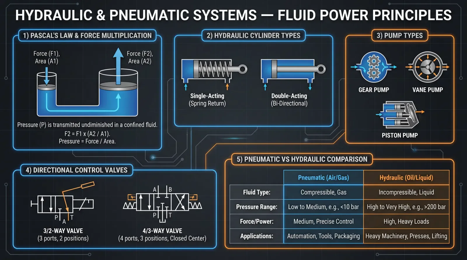
Fluid power harnesses the energy stored in pressurized fluids—liquids for hydraulics, gases (usually air) for pneumatics—to perform mechanical work. This chapter codifies the fundamental laws, enabling you to design, operate, and maintain systems with the precision demanded by the Practitioner order.
1. Fluid Properties and Behavior
Understanding fluid properties is the cornerstone of fluid power mastery. Below, Table 1 encapsulates essential fluid properties for common hydraulic and pneumatic fluids.
Table 1: Fluid Properties Relevant to Fluid Power Systems
| Property | Hydraulic Oil (ISO VG 46) | Water (Distilled) | Compressed Air (Dry) | Nitrogen (Dry) |
|---|---|---|---|---|
| Density (kg/m³) | 870 | 1000 | 1.225 | 1.165 |
| Dynamic Viscosity (mPa·s) | 46 | 1 | 0.018 | 0.017 |
| Bulk Modulus (MPa) | 1400 | 2100 | 0.14 (approx.) | 0.15 (approx.) |
| Vapor Pressure (kPa) | <0.1 | 2.3 | — | — |
| Operating Temperature Range (°C) | -20 to 80 | 0 to 100 | -20 to 60 | -20 to 60 |
2. Fundamental Fluid Power Equations
Memorize these core equations; they govern system design and performance calculations.
- Continuity Equation: \( Q = A \times v \)
Q = volumetric flow rate (m³/s), A = cross-sectional area (m²), v = fluid velocity (m/s)
- Bernoulli’s Equation (simplified for incompressible fluids):
\( P_1 + \frac{1}{2} \rho v_1^2 + \rho g h_1 = P_2 + \frac{1}{2} \rho v_2^2 + \rho g h_2 + h_f \) P = pressure (Pa), ρ = density (kg/m³), v = velocity (m/s), g = gravity (9.81 m/s²), h = elevation height (m), h_f = head loss (m)
- Pascal’s Law: Pressure applied to an enclosed fluid is transmitted undiminished:
\( F = P \times A \) F = force (N), P = pressure (Pa), A = area (m²)
- Power Equation:
\( P_{hydraulic} = P \times Q \) Power (W) = pressure (Pa) × flow rate (m³/s)
3. Fluid Power System Types
- Open-Center Systems: Continuous flow; excess fluid returns to the reservoir without routing through actuators unless commanded.
- Closed-Center Systems: Flow stops when actuators are inactive; pressure maintained in the circuit.
- Hydrostatic Systems: Use of pumps and motors with variable displacement for precise control.
Chapter II: Hydraulic System Components
This chapter unlocks detailed knowledge on system components, their selection, and integration.
1. Pumps
Pumps convert mechanical energy into hydraulic energy. Selection criteria prioritize flow rate, pressure capability, efficiency, and fluid compatibility.
Table 2: Pump Types and Characteristics
| Pump Type | Max Pressure (MPa) | Typical Flow Range (L/min) | Efficiency (%) | Notes |
|---|---|---|---|---|
| Gear Pump | 14 | 5 – 150 | 85 – 90 | Simple, robust; moderate efficiency |
| Vane Pump | 14 | 10 – 200 | 85 – 90 | Smoother flow; sensitive to contamination |
| Piston Pump | 35 | 5 – 500 | 90 – 95 | High pressure, precise control |
2. Valves
Valves regulate flow, pressure, and direction. Their correct selection dictates system responsiveness and safety.
Table 3: Valve Types and Functions
| Valve Type | Function | Control Method | Typical Pressure Rating (MPa) | Application Notes |
|---|---|---|---|---|
| Directional Control | Direct fluid path | Manual, Solenoid | 14 – 35 | Controls actuator movement direction |
| Pressure Relief | Limits system pressure | Spring-loaded | 7 – 35 | Prevents overpressure |
| Flow Control | Regulates flow rate | Adjustable or fixed | 7 – 21 | Controls actuator speed |
| Check Valve | Allows flow in one direction only | Passive (spring) | 14 – 35 | Prevents backflow |
3. Actuators
Actuators convert fluid power back to mechanical work.
- Hydraulic Cylinders: Linear motion, high force
- Hydraulic Motors: Rotary motion, variable torque and speed
4. Reservoirs
Reservoirs store fluid, dissipate heat, and allow air separation. Design includes capacity for fluid volume plus 25% reserve.
5. Filters
Filters remove contaminants that degrade system performance.
- Micron ratings: 3–25 μm typical for hydraulic systems
- Placement: Suction line, pressure line, return line
Chapter III: Pneumatics Components Overview
Pneumatics is governed by similar principles but requires specialized components due to fluid compressibility.
1. Compressors
Compressors generate compressed air.
| Compressor Type | Output Pressure (MPa) | Flow Rate (L/min) | Notes |
|---|---|---|---|
| Reciprocating | 0.7 – 1.0 | 50 – 300 | High pressure, intermittent |
| Rotary Screw | 0.7 – 1.0 | 100 – 1000 | Continuous, quieter |
2. Air Preparation Units
- Filters: Remove particles and moisture
- Regulators: Maintain constant pressure
- Lubricators: Add controlled oil mist for component longevity
3. Actuators
- Pneumatic Cylinders: Linear motion, fast response
- Pneumatic Motors: Rotary, lower torque than hydraulic equivalents
Chapter IV: Designing Hydraulic Circuits – Protocol
The faithful apprentice must master circuit design to ensure efficient, safe, and reliable operation. Follow these exact steps:
Step 1: Define System Requirements
- Identify actuator types and required forces/motion.
- Determine operating pressures and flow rates.
- Specify environmental constraints (temperature, contamination risk).
Step 2: Calculate Flow Rate and Pressure
- Calculate force required by actuators using: \( F = P \times A \) (Area of piston known from actuator specs)
- Determine flow rate from actuator speed: \( Q = A \times v \) (v = desired velocity in m/s)
- Add 10–15% safety margin for inefficiencies and losses.
Step 3: Select Pump
- Match calculated flow and pressure to pump rated specifications (see Table 2).
- Choose pump type (gear, vane, piston) based on application requirements.
Step 4: Choose Valves
- Select directional control valves compatible with flow and pressure.
- Include pressure relief valves set 10% above max operating pressure.
- Implement flow control valves where speed regulation is critical.
Step 5: Layout Circuit
- Sketch schematic including reservoir, pump, valves, actuators.
- Include pressure gauges at key points.
- Use appropriate line sizes to avoid excessive pressure drop (refer to Volume VII: Fluid Dynamics).
Step 6: Select Hydraulic Fluid
- Choose fluid compatible with operating temperature and materials.
- Confirm viscosity matches pump and system recommendations.
Step 7: Assemble and Test
- Assemble components per manufacturer torque and alignment specs.
- Perform leak test: pressurize system to max operating pressure and monitor for pressure drop over 30 minutes.
- Cycle actuators and verify smooth operation.
Chapter V: Troubleshooting Hydraulic Leaks – Protocol

Leaks degrade efficiency and cause hazards. Follow this precise protocol to locate and repair leaks.
Step 1: Safety Precautions
- Depressurize system fully before inspection.
- Wear protective gloves and eye protection.
Step 2: Visual Inspection
- Examine hose connections, fittings, seals, and cylinders.
- Note wet spots, drips, or residue.
Step 3: Use Leak Detection Fluid
- Apply approved leak detection fluid or soap solution to suspect areas.
- Observe for bubble formation under pressure.
Step 4: Tighten Connections
- Use torque wrench to tighten fittings to manufacturer specifications (see Table 4).
- Avoid over-tightening which can cause damage.
Step 5: Replace Damaged Components
- Replace hoses with rated equivalents matching pressure and temperature.
- Replace seals with OEM parts.
Step 6: System Test
- Repressurize and monitor for leaks over 60 minutes.
- Record pressure readings at intervals (every 15 minutes).
Table 4: Recommended Torque Values for Hydraulic Fittings
| Fitting Size (in) | Torque (N·m) |
|---|---|
| 1/4" | 20 – 25 |
| 3/8" | 35 – 45 |
| 1/2" | 60 – 70 |
| 3/4" | 110 – 130 |
| 1" | 180 – 220 |
Chapter VI: Selecting Pumps and Valves – Detailed Specifications
The following tables guide precise component selection.
Table 5: Hydraulic Pump Selection Guide
| Application Type | Required Pressure (MPa) | Flow Rate (L/min) | Recommended Pump Type | Notes |
|---|---|---|---|---|
| Mobile Equipment | 14 – 21 | 20 – 100 | Gear or Vane | Robust, cost-effective |
| Industrial Presses | 21 – 35 | 5 – 50 | Piston | High pressure, precise control |
| Injection Molding | 21 – 35 | 50 – 200 | Variable Displacement | Energy efficient |
Table 6: Valve Selection Guide
| Valve Function | Max Flow (L/min) | Max Pressure (MPa) | Control Type | Material |
|---|---|---|---|---|
| Directional Control | 10 – 200 | 14 – 35 | Manual, Solenoid | Steel or Aluminum |
| Pressure Relief | N/A | 7 – 35 | Spring-loaded | Steel |
| Flow Control | 5 – 150 | 7 – 21 | Adjustable Needle | Brass or Steel |
| Check Valve | 10 – 200 | 14 – 35 | Spring-loaded | Steel |
Chapter VII: Maintenance Schedules
Adherence to maintenance schedules is mandatory to prevent catastrophic failures.
| Component | Inspection Frequency | Maintenance Actions | Replacement Interval |
|---|---|---|---|
| Hydraulic Pump | Monthly | Check noise, vibration, temperature | Every 5000 hours |
| Valves | Monthly | Inspect seals, test operation | Every 10000 hours |
| Hydraulic Hoses | Weekly | Visual check for cracks, bulges | Every 5 years or upon damage |
| Filters | Weekly | Replace or clean per pressure drop indication | Every 250 hours |
| Reservoir | Quarterly | Drain sediment, check fluid level and quality | Every 2 years |
Chapter VIII: Safety Guidelines
Absolute adherence to these safety protocols is non-negotiable.
- Always depressurize before disassembly.
- Use rated personal protective equipment (PPE).
- Avoid loose clothing near moving components.
- Never bypass pressure relief valves.
- Store hydraulic fluids in sealed, labeled containers.
- Dispose of contaminated fluids per environmental regulations.
- Maintain clean work environment to prevent contamination.
- Follow lockout/tagout procedures during maintenance.
End of Volume V: Hydraulics and Pneumatics Fundamentals
The sacred knowledge herein is the foundation of all fluid power mastery. Guard it well, apply it without hesitation, and pass it only to those worthy. For continued learning on fluid dynamics and filtration systems, refer to Volume VII: Fluid Dynamics and Volume IX: Filtration Mastery, respectively.
<!-- SECTION 25 -->
Volume VI: Microcontroller Fundamentals and Programming
Chapter I: Architectural Foundations of Arduino and ESP32 Platforms

The mastery of microcontroller platforms is indispensable for the technologist. This chapter imparts the sacred knowledge of two paramount architectures: Arduino and ESP32. Their structural and functional understanding forms the cornerstone of all embedded systems and automation projects.
1. Arduino Architecture Overview
The Arduino platform primarily revolves around the ATmega328P microcontroller (for Arduino Uno), a robust 8-bit AVR RISC architecture designed for embedded control.
| Feature | Specification |
|---|---|
| MCU Core | 8-bit AVR RISC |
| Clock Speed | 16 MHz |
| Flash Memory | 32 KB (0.5 KB used by bootloader) |
| SRAM | 2 KB |
| EEPROM | 1 KB |
| Digital I/O Pins | 14 (6 PWM capable) |
| Analog Input Pins | 6 |
| Operating Voltage | 5V |
| Communication Interfaces | UART, SPI, I2C |
Structural Components:
- CPU Core: Executes instructions.
- Flash Memory: Stores program code.
- SRAM: Temporary data storage.
- EEPROM: Non-volatile data storage.
- I/O Ports: Interface points with external world.
2. ESP32 Architecture Overview
The ESP32 is a 32-bit dual-core microcontroller, integrating WiFi and Bluetooth capabilities, designed for advanced IoT applications.
| Feature | Specification |
|---|---|
| MCU Core | Dual-core Tensilica LX6, 32-bit |
| Clock Speed | Up to 240 MHz |
| Flash Memory | External, typically 4 MB or more |
| SRAM | 520 KB |
| Operating Voltage | 3.3V |
| Digital I/O Pins | 34 |
| Analog Input Pins | 18 (12-bit ADC) |
| Communication Interfaces | UART (3), SPI (4), I2C (2), CAN, Ethernet MAC |
| Wireless Connectivity | WiFi 802.11 b/g/n, Bluetooth v4.2 BR/EDR and BLE |
Key Functional Blocks:
- CPU Cores: Handle multitasking and real-time operations.
- WiFi/Bluetooth Modules: Enable wireless communication.
- RTC: Real-Time Clock for time-keeping in low-power mode.
- Peripheral Interfaces: Rich set for sensor and actuator integration.
Chapter II: Input/Output Interfacing and Sensor Integration
This chapter unveils the sacred protocols for interfacing microcontrollers with the external world through sensors and actuators.
1. Digital and Analog I/O Pin Functionality
Both Arduino and ESP32 platforms possess configurable pins divided into:
- Digital Input/Output Pins: Detect or generate digital signals (HIGH/LOW).
- Analog Input Pins: Read continuous voltage values.
- PWM Output: Simulate analog output via pulse width modulation.
2. Pinout Tables
Arduino Uno Pinout Summary
| Pin Number | Type | Functionality | Notes |
|---|---|---|---|
| 0 (RX) | Digital I/O | UART Receive | Serial communication |
| 1 (TX) | Digital I/O | UART Transmit | Serial communication |
| 2 - 13 | Digital I/O | General purpose I/O | Pins 3, 5, 6, 9, 10, 11 support PWM |
| A0 - A5 | Analog Input | Analog to Digital Converter (ADC) | 10-bit resolution |
| RESET | Control | Resets MCU | Active LOW |
| 5V | Power | 5 Volt supply | Regulated output |
| GND | Power | Ground | Common ground |
ESP32 Pinout Summary (Typical DevKitC Board)
| Pin Number | Type | Functionality | Notes |
|---|---|---|---|
| GPIO0 | Digital I/O | Boot mode selection, input | Must be LOW during boot to enter flash mode |
| GPIO1 (TX) | Digital I/O | UART Transmit | Serial communication |
| GPIO3 (RX) | Digital I/O | UART Receive | Serial communication |
| GPIO4 | Digital I/O | General Purpose | Can be used for I2C, SPI, PWM |
| GPIO12-15 | Digital I/O | General Purpose | Some pins have strapping functions |
| GPIO34-39 | Analog Input | ADC channels | Input only, no output |
| EN | Control | Enable pin | Reset MCU when pulled LOW |
| 3.3V | Power | 3.3 Volt supply | Regulated output |
| GND | Power | Ground | Common ground |
3. Sensor Integration: Protocols and Calibration
Sensors require precise interfacing and calibration to produce reliable data.
Common Sensor Protocols
| Protocol | Description | Physical Interface | Supported by Arduino | Supported by ESP32 |
|---|---|---|---|---|
| I2C | Inter-Integrated Circuit | SDA, SCL (2 wires) | Yes | Yes |
| SPI | Serial Peripheral Interface | MOSI, MISO, SCLK, CS | Yes | Yes |
| UART | Universal Asynchronous Receiver/Transmitter | TX, RX | Yes | Yes |
| Analog | Analog Voltage Output | Analog input pin | Yes | Yes |
4. Sensor Calibration Protocol
To ensure sensor output matches physical parameters, calibration is mandatory.
Example: Calibrating a DHT22 Temperature and Humidity Sensor
| Step | Procedure |
|---|---|
| 1 | Connect sensor data pin to Arduino digital pin 2 |
| 2 | Power sensor with 3.3V (ESP32) or 5V (Arduino) |
| 3 | Use library DHT.h to initialize sensor |
| 4 | Read raw temperature and humidity values |
| 5 | Compare sensor output to a reference thermometer/hygrometer |
| 6 | Calculate offset: Offset = Reference value - Sensor value |
| 7 | Apply offset correction in software by adding offset to readings |
| 8 | Repeat steps 4-7 under different environmental conditions |
Chapter III: Compiling and Uploading Code
This chapter provides the exact, stepwise ritual to convert your sacred code into executable instructions within the microcontroller.
1. Arduino Platform Compilation and Upload Protocol
Prerequisites
- Arduino IDE (latest version)
- USB connection cable (Type A to B or Micro USB)
- Correct board and port selected
Step-by-step Compilation and Upload
- Install Arduino IDE from [https://www.arduino.cc/en/software](https://www.arduino.cc/en/software).
- Connect Arduino board via USB cable to your computer.
- Launch Arduino IDE.
- Navigate to Tools > Board > Arduino Uno (or your specific board).
- Navigate to Tools > Port and select the COM port associated with the Arduino.
- Open or write your code in the IDE editor.
- Click Verify (checkmark icon) to compile code.
- Observe the output console for any errors; resolve as needed.
- Click Upload (right-arrow icon) to transfer the compiled binary to the Arduino.
- Wait for confirmation message: "Done uploading."
- Open Serial Monitor (Tools > Serial Monitor) to view debug output, if applicable.
2. ESP32 Platform Compilation and Upload Protocol
Prerequisites
- Arduino IDE with ESP32 board support installed
- USB cable (usually Micro USB or USB-C)
- USB-to-Serial driver installed (if required)
ESP32 Board Support Installation
- Open Arduino IDE.
- Navigate to File > Preferences.
- In the Additional Boards Manager URLs field, add:
https://dl.espressif.com/dl/package_esp32_index.json - Click OK.
- Navigate to Tools > Board > Boards Manager.
- Search for "esp32", select esp32 by Espressif Systems, and click Install.
- Restart Arduino IDE.
Upload Steps
- Connect ESP32 board via USB.
- In Arduino IDE, select Tools > Board > ESP32 Dev Module.
- Select the appropriate COM port under Tools > Port.
- Write or open your sketch.
- Click Verify to compile.
- Press and hold the BOOT button on the ESP32.
- Click Upload.
- Release the BOOT button when upload begins.
- Wait for "Done uploading" confirmation.
- Use Serial Monitor to observe output.
Chapter IV: Actuator Control and Automation Projects
Understanding actuator control is a sacred skill, enabling the microcontroller to influence the physical realm.
1. Actuator Types and Control Methods
| Actuator Type | Control Signal Type | Interface Method | Notes |
|---|---|---|---|
| DC Motor | PWM or Digital | Motor Driver (H-Bridge) | Use external driver for current |
| Servo Motor | PWM (50 Hz) | Direct PWM pin | Position control via pulse width |
| Stepper Motor | Digital | Stepper driver or direct pins | Requires sequence of pulses |
| Relay | Digital | Digital pin via transistor | Controls high-voltage loads |
| Solenoid | Digital/PWM | Driver circuit | Requires external power supply |
2. Protocol for Controlling a Servo Motor with Arduino
Materials:
- Arduino Uno
- Servo motor (e.g., SG90)
- Jumper wires
- External 5V power supply (if servo current exceeds Arduino limits)
Procedure:
- Connect servo signal wire to Arduino digital pin 9.
- Connect servo power wire to 5V power supply.
- Connect servo ground wire to common ground with Arduino.
- Include the servo library:
#include <Servo.h>. - Instantiate servo object:
Servo myServo;. - In
setup(), attach servo:myServo.attach(9);. - In
loop(), write position:myServo.write(angle);where angle is 0 to 180. - Upload code using the compilation/upload protocol.
- Observe servo movement corresponding to angle commands.
3. Sample Automation Project: Temperature-Controlled Fan
Objective: Automatically activate a fan when temperature exceeds a threshold.
Components:
- Arduino Uno
- DHT11 Temperature sensor
- DC fan (5V)
- NPN Transistor (e.g., 2N2222)
- Flyback diode (1N4001)
- Resistors: 1 kΩ base resistor
- Power supply
Wiring:
| Component | Connection |
|---|---|
| DHT11 Data Pin | Arduino digital pin 2 |
| Fan positive | 5V power supply |
| Fan negative | Collector of NPN transistor |
| Emitter of transistor | Ground |
| Base of transistor | Arduino digital pin 9 via 1 kΩ resistor |
| Flyback diode | Across fan terminals (cathode to +5V) |
| Common ground | Connect all grounds |
Code Logic:
- Initialize DHT11 sensor.
- Read temperature periodically.
- If temperature > threshold (e.g., 30°C), set digital pin 9 HIGH (activate transistor, fan ON).
- Else, set pin LOW (fan OFF).
Step-by-step Implementation:
- Assemble hardware as per wiring table.
- Include
DHT.hand define pins. - In
setup(), initialize sensor and set pin 9 as output. - In
loop(), read temperature, compare with threshold. - Control pin 9 accordingly.
- Upload code via Arduino IDE.
- Test by heating sensor area or using a heat source.
Chapter V: Programming Libraries and Sensor Specifications
1. Essential Programming Libraries
| Library | Supported Platforms | Functionality | Installation Source |
|---|---|---|---|
DHT | Arduino, ESP32 | Interface DHT11, DHT22 temperature/humidity sensors | Arduino Library Manager |
Servo | Arduino | Control servo motors | Arduino Library Manager |
Wire | Arduino, ESP32 | I2C communication | Pre-installed |
SPI | Arduino, ESP32 | SPI communication | Pre-installed |
WiFi | ESP32 | WiFi networking | ESP32 Arduino core |
BluetoothSerial | ESP32 | Bluetooth serial communication | ESP32 Arduino core |
2. Sensor Specifications Table (Common Sensors)
| Sensor Model | Type | Interface | Operating Voltage | Measurement Range | Accuracy | Comments |
|---|---|---|---|---|---|---|
| DHT11 | Temperature/Humidity | Digital | 3.3V - 5V | Temp: 0-50°C, Humidity: 20-90% RH | ±2°C, ±5% RH | Low cost, slow response |
| DHT22 | Temperature/Humidity | Digital | 3.3V - 6V | Temp: -40 to 80°C, Humidity: 0-100% RH | ±0.5°C, ±2-5% RH | Higher precision than DHT11 |
| BMP280 | Pressure/Temp | I2C/SPI | 1.71V - 3.6V | 300-1100 hPa, -40 to 85°C | ±1 hPa, ±1°C | Compact, low-power |
| MQ-2 | Gas (Smoke, LPG) | Analog | 5V | 200-10000 ppm | Varies by gas | Requires calibration |
| HC-SR04 | Ultrasonic Distance | Digital | 5V | 2 cm - 400 cm | ±3 mm | Requires trigger and echo pins |
Chapter VI: Advanced Example Projects
Project 1: WiFi-Enabled Environmental Monitor (ESP32)
Objective: Measure temperature and humidity, transmit data via WiFi.
Components:
- ESP32 Development Board
- DHT22 Sensor
- USB cable for power and programming
- WiFi network credentials
Step-by-step Procedure:
- Connect DHT22 data pin to GPIO4 on ESP32.
- Power sensor from 3.3V pin.
- Connect grounds together.
- Install libraries:
DHT.h,WiFi.h. - Use example code below:
#include <WiFi.h>
#include "DHT.h"

#define DHTPIN 4
#define DHTTYPE DHT22

const char* ssid = "YourSSID";
const char* password = "YourPassword";

DHT dht(DHTPIN, DHTTYPE);

void setup() {
  Serial.begin(115200);
  dht.begin();
  WiFi.begin(ssid, password);
  while (WiFi.status() != WL_CONNECTED) {
    delay(500);
    Serial.print(".");
  }
  Serial.println("WiFi connected");
}

void loop() {
  float h = dht.readHumidity();
  float t = dht.readTemperature();

  if (isnan(h) || isnan(t)) {
    Serial.println("Failed to read from DHT sensor!");
    return;
  }

  Serial.print("Humidity: ");
  Serial.print(h);
  Serial.print(" %\t");
  Serial.print("Temperature: ");
  Serial.print(t);
  Serial.println(" *C");

  delay(2000);
}- Upload code using ESP32 upload protocol.
- Open serial monitor to verify sensor readings and WiFi connection.
Project 2: Automated Plant Watering System (Arduino)
Objective: Measure soil moisture; activate pump when soil is dry.
Components:
- Arduino Uno
- Soil Moisture Sensor (analog output)
- Relay Module (5V)
- Water pump (5V)
- Power supply
Wiring Instructions:
| Component | Arduino Pin | Notes |
|---|---|---|
| Soil Sensor VCC | 5V | Power sensor |
| Soil Sensor GND | GND | Common ground |
| Soil Sensor Analog Output | A0 | Analog sensor reading |
| Relay IN | Digital pin 8 | Controls relay |
| Relay VCC | 5V | Relay power |
| Relay GND | GND | Common ground |
| Pump + | Relay Normally Open (NO) contact | Power supply through relay |
| Pump - | Power supply GND | - |
Step-by-step Code Implementation:
- Set pin modes: A0 input, pin 8 output.
- Read analog value from soil sensor.
- Define soil moisture threshold (e.g., 400 analog units).
- If reading below threshold (dry soil), set pin 8 HIGH (activate relay).
- Else, set pin 8 LOW (deactivate relay).
- Add delay to avoid excessive pump cycling.
Sample Code:
const int soilPin = A0;
const int relayPin = 8;
const int threshold = 400;

void setup() {
  pinMode(relayPin, OUTPUT);
  digitalWrite(relayPin, LOW);
  Serial.begin(9600);
}

void loop() {
  int soilMoisture = analogRead(soilPin);
  Serial.print("Soil Moisture: ");
  Serial.println(soilMoisture);

  if (soilMoisture < threshold) {
    digitalWrite(relayPin, HIGH); // Pump ON
  } else {
    digitalWrite(relayPin, LOW);  // Pump OFF
  }
  delay(2000);
}- Upload code via Arduino IDE.
- Test system by drying soil and observing pump activation.
Summary
This volume has meticulously transmitted the essential knowledge for mastery over Arduino and ESP32 microcontrollers, emphasizing architecture, I/O interfacing, sensor calibration, actuator control,
<!-- SECTION 26 -->
Volume VI: Sensor Technologies and Data Acquisition
Chapter I: Overview of Sensor Technologies

In the sacred pursuit of mastering the art of data acquisition, the foundation lies in understanding the sensor—an instrument of conversion, transforming physical phenomena into electrical signals. This volume unveils the essential sensor types—temperature, humidity, proximity, and light—and delivers comprehensive protocols for wiring, calibration, and data logging. The knowledge contained herein is a living flame, illuminating the path from raw phenomena to actionable data.
Section 1: Temperature Sensors
1.1 Types and Characteristics
Temperature measurement is the cornerstone of environmental and process control. Four primary sensor types dominate the field:
| Sensor Type | Operating Principle | Accuracy Range | Response Time (s) | Output Type | Typical Application |
|---|---|---|---|---|---|
| Thermocouple | Seebeck effect voltage | ±1°C to ±5°C | 0.5 - 2 | Millivolts (mV) | High-temperature, industrial |
| RTD (Pt100) | Resistance change (Platinum) | ±0.1°C to ±0.5°C | 0.5 - 1 | Resistance (Ω) | Precision laboratory and industry |
| Thermistor (NTC) | Resistance change (Semiconductor) | ±0.1°C to ±2°C | 0.1 - 0.5 | Resistance (Ω) | HVAC, medical devices |
| Semiconductor IC | Bandgap voltage variation | ±0.5°C to ±2°C | 0.1 - 0.3 | Analog voltage (0-5V) | Embedded systems, microcontrollers |
1.2 Wiring Protocols
Thermocouple Wiring
- Obtain thermocouple wire matching the sensor type (e.g., Type K: Chromel-Alumel).
- Connect thermocouple leads to the signal conditioning unit or ADC input with cold-junction compensation.
- Use twisted pair wiring, shielded against electromagnetic interference.
- Maintain polarity: positive lead to positive terminal, negative to negative terminal.
- Avoid junctions with dissimilar metals beyond the sensor tip to prevent parasitic voltages.
RTD Wiring
- Use a 3-wire or 4-wire configuration for high accuracy.
- Connect one lead to the excitation voltage source.
- Connect the other leads to the differential input of a high-precision ADC or Wheatstone bridge.
- Use shielded cable and place the sensor in thermal contact with the measured object.
- Calibrate to account for lead resistance.
Thermistor Wiring
- Connect thermistor in a voltage divider circuit with a precision resistor of known value.
- Use a stable power supply (e.g., 5V regulated).
- Connect the output node between thermistor and resistor to an ADC input.
- Employ shielded twisted pair wiring.
- Minimize self-heating by limiting current to less than 1 mA.
Semiconductor IC Sensor Wiring
- Connect power pins to regulated supply (typically 5V or 3.3V).
- Connect analog output to ADC input on microcontroller.
- Connect ground pins to common system ground.
- Implement decoupling capacitors (0.1 µF ceramic) near the sensor pins.
- Place sensor in environment representative of measurement target.
1.3 Calibration Procedure
Calibration of Thermistor Sensor
Materials Required:
- Precision temperature source (e.g., temperature-controlled bath)
- Reference thermometer with ±0.05°C accuracy
- Multimeter or data acquisition system with ADC
Steps:
- Immerse the thermistor and reference thermometer in the temperature-controlled bath.
- Set bath temperature to first calibration point (e.g., 0°C).
- Allow thermal equilibrium for 5 minutes.
- Record thermistor voltage (V_thermistor) and reference temperature (T_ref).
- Increase bath temperature in 10°C increments up to 100°C, repeating steps 3-4.
- For each point, calculate resistance R = (V_supply / V_thermistor - 1) * R_fixed.
- Fit resistance-temperature data to Steinhart-Hart equation:
\[ \frac{1}{T} = A + B \ln R + C (\ln R)^3 \]
where \(T\) is temperature in Kelvin.
- Store coefficients A, B, C in microcontroller memory for real-time conversion.
1.4 Data Logging Protocol
- Initialize ADC with 12-bit resolution or higher.
- Acquire voltage sample from sensor at desired frequency (typically 1 Hz for environmental monitoring).
- Convert ADC counts to temperature using calibration curve.
- Timestamp data with real-time clock (RTC) module.
- Store data in non-volatile memory (EEPROM or SD card).
- For continuous logging, implement circular buffer with overflow protection.
Section 2: Humidity Sensors
2.1 Types and Characteristics
Humidity sensors quantify water vapor concentration by measuring relative humidity (RH) or absolute humidity. Principal sensor types:
| Sensor Type | Operating Principle | Accuracy Range | Response Time (s) | Output Type | Typical Applications |
|---|---|---|---|---|---|
| Capacitive | Change in dielectric constant | ±2% RH | 8 - 15 | Analog voltage / I2C | HVAC, weather stations |
| Resistive | Change in resistance with moisture | ±3% RH | 10 - 20 | Analog voltage | Industrial control |
| Thermal Conductivity | Change in thermal conductivity | ±3% RH | 1 - 5 | Voltage/current | Process control |
| Dew Point | Chilled mirror condensation | ±0.1°C dew point | 5 - 10 | Digital output | Meteorology, calibration |
2.2 Wiring Protocols
Capacitive Sensor Wiring
- Connect Vcc to regulated 3.3V or 5V supply as per sensor datasheet.
- Connect output pin (analog or digital) to microcontroller ADC or digital input.
- Connect ground to system ground.
- Include a 0.1 µF bypass capacitor close to Vcc and ground pins.
- Avoid placing sensor near heat sources or moisture traps.
Resistive Sensor Wiring
- Connect sensor in series with a precision resistor to form a voltage divider.
- Supply regulated voltage to the voltage divider.
- Connect the midpoint between sensor and resistor to ADC input.
- Use shielded cable to reduce noise.
- Ensure sensor is exposed to airflow representative of environment.
2.3 Calibration Procedure
Capacitive Humidity Sensor Calibration
Materials:
- Saturated salt solutions for fixed known RH points (see Table 2.3.1)
- Precision hygrometer for reference
| Salt Solution | Approximate RH at 25°C (%) |
|---|---|
| Lithium Chloride (LiCl) | 11.3 |
| Magnesium Chloride | 33.1 |
| Sodium Chloride (NaCl) | 75.3 |
| Potassium Nitrate | 93.6 |
Steps:
- Place sensor and reference hygrometer inside sealed container with salt solution.
- Allow system to stabilize for 24 hours at 25°C.
- Record sensor output voltage and reference RH.
- Repeat for each salt solution.
- Generate linear or polynomial fit between sensor output and RH.
- Program calibration coefficients into microcontroller.
2.4 Data Logging Protocol
- Configure ADC input channel for sensor voltage.
- Sample sensor output every 1-10 seconds.
- Convert voltage to RH using calibration curve.
- Store data with timestamp in non-volatile memory.
- Implement alert thresholds for humidity limits.
Section 3: Proximity Sensors
3.1 Types and Characteristics
Proximity sensors detect the presence or absence of objects without physical contact. Categories include:
| Sensor Type | Operating Principle | Sensing Range | Response Time (ms) | Output Type | Typical Applications |
|---|---|---|---|---|---|
| Inductive | Eddy current variation in metal | 1-30 mm | 1-5 | Digital | Metal detection |
| Capacitive | Change in capacitance | 1-50 mm | 1-10 | Digital/Analog | Non-metal object detection |
| Ultrasonic | Time of flight of sound waves | 2 cm - 4 m | 10-50 | Digital | Distance measurement |
| Infrared (IR) | Reflection of IR light | 2 cm - 80 cm | 10-50 | Digital | Object detection, counting |
3.2 Wiring Protocols
Inductive Proximity Sensor Wiring
- Connect power supply pins to 12-24V DC regulated source.
- Connect sensor output (PNP or NPN) to microcontroller input with pull-up or pull-down resistor as required.
- Connect sensor ground to system ground.
- Use shielded cable and maintain distance from high-current lines.
- Verify sensor output polarity and logic level.
Ultrasonic Sensor Wiring (HC-SR04 Example)
- Connect Vcc to 5V regulated supply.
- Connect GND to system ground.
- Connect Trigger pin to microcontroller digital output.
- Connect Echo pin to microcontroller digital input.
- Use short, twisted pair wiring to minimize noise.
3.3 Calibration Procedure
Ultrasonic Sensor Distance Calibration
Materials:
- Precision ruler or laser distance meter
- Flat, reflective surface
Steps:
- Place sensor on stable surface.
- Position reflective target at known distances (e.g., 10 cm, 50 cm, 100 cm).
- Issue trigger pulse and measure echo pulse width.
- Calculate distance \( d = \frac{t \times v}{2} \), where \( t \) is time in seconds, \( v \) speed of sound (343 m/s at 20°C).
- Compare calculated distance to reference.
- Generate correction factor for temperature or environmental conditions.
- Program correction into microcontroller.
3.4 Data Logging Protocol
- Generate trigger pulse of 10 µs duration on Trigger pin.
- Measure time duration of Echo pin high state.
- Convert duration to distance using calibration.
- Timestamp and store distance data.
- Implement filtering algorithms (e.g., moving average) to reduce noise.
Section 4: Light Sensors
4.1 Types and Characteristics
Light sensors measure luminous intensity or irradiance. Common types:
| Sensor Type | Operating Principle | Spectral Range (nm) | Response Time (ms) | Output Type | Typical Applications |
|---|---|---|---|---|---|
| Photodiode | Photocurrent proportional to light | 400-1100 | <1 | Current/Voltage | Optical communication, ambient light |
| Phototransistor | Photocurrent with internal gain | 400-1100 | 1-10 | Current/Voltage | Light detection, switches |
| LDR (CdS cell) | Resistance change with light intensity | 400-700 | 10-100 | Resistance | Light level sensing |
| Ambient Light Sensor IC | Integrated photodiode + ADC | Visible spectrum | 100-300 | Digital (I2C) | Display brightness control |
4.2 Wiring Protocols
Photodiode Wiring
- Connect photodiode in photoconductive mode: cathode to positive supply, anode to virtual ground input of transimpedance amplifier.
- Use low-noise operational amplifier with feedback resistor for current-to-voltage conversion.
- Power amplifier with dual supply ±12V or single supply with rail-to-rail op-amp.
- Add small feedback capacitor (pF range) for stability.
- Shield sensor and amplifier from ambient electromagnetic interference.
LDR Wiring
- Connect LDR in series with a fixed resistor to form a voltage divider.
- Supply regulated voltage (3.3V or 5V).
- Connect voltage divider output to ADC input.
- Use shielded cable.
- Minimize ambient temperature variations to reduce resistance drift.
Ambient Light Sensor IC Wiring
- Connect Vcc to 3.3V regulated supply.
- Connect ground to system ground.
- Connect SDA and SCL lines to microcontroller I2C bus with pull-up resistors (4.7 kΩ).
- Place sensor on PCB with unobstructed view to ambient light.
- Include 0.1 µF decoupling capacitor near sensor.
4.3 Calibration Procedure
Photodiode Calibration
Materials:
- Calibrated light source with known luminous intensity (lux)
- Lux meter for reference
Steps:
- Position photodiode sensor and lux meter side by side.
- Illuminate sensor with known lux levels (e.g., 100, 500, 1000, 5000 lx).
- Measure photodiode output voltage/current at each level.
- Plot sensor output vs. lux.
- Fit linear or polynomial curve.
- Store calibration data in microcontroller.
4.4 Data Logging Protocol
- Sample photodiode voltage with high-resolution ADC (16-bit preferred).
- Convert voltage to lux using calibration curve.
- Timestamp and store data.
- Use averaging filter to reduce noise.
- Implement saturation detection to prevent data corruption at high intensities.
Section 5: Integration Examples with Microcontrollers
This section provides detailed step-by-step guides to integrate sensors with microcontrollers, focusing on Arduino Uno (ATmega328P) and STM32F103 platforms.
5.1 Arduino Uno Integration for Temperature and Humidity (DHT22 Sensor Example)
The DHT22 is a combined digital temperature and humidity sensor.
Materials:
- Arduino Uno board
- DHT22 sensor
- 4.7 kΩ pull-up resistor
- Breadboard, jumper wires
Wiring Steps:
- Connect sensor Vcc to Arduino 5V pin.
- Connect sensor GND to Arduino GND.
- Connect sensor data pin to Arduino digital pin 2.
- Place 4.7 kΩ resistor between data pin and 5V line.
- Verify connections.
Software Setup:
- Install DHT sensor library from Adafruit.
- Initialize sensor in code:
#include "DHT.h"
#define DHTPIN 2
#define DHTTYPE DHT22
DHT dht(DHTPIN, DHTTYPE);

void setup() {
  Serial.begin(9600);
  dht.begin();
}

void loop() {
  float humidity = dht.readHumidity();
  float temperature = dht.readTemperature();

  if (isnan(humidity) || isnan(temperature)) {
    Serial.println("Failed to read from DHT sensor!");
    return;
  }

  Serial.print("Humidity: ");
  Serial.print(humidity);
  Serial.print("%  Temperature: ");
  Serial.print(temperature);
  Serial.println("°C");
  delay(2000);
}
Data Logging:
- Connect Arduino to PC via USB.
- Use serial terminal software to capture data.
- For onboard logging, attach SD card module and implement file write operations.
5.2 STM32F103 Integration for Ultrasonic Distance Measurement (HC-SR04)
Materials:
- STM32F103 "Blue Pill"
- HC-SR04 ultrasonic sensor
- Jumper wires, breadboard
Wiring Steps:
- Connect Vcc on HC-SR04 to 5V supply.
- Connect GND to STM32 GND.
- Connect Trigger pin to STM32 GPIO pin PA1.
- Connect Echo pin to STM32 GPIO pin PA2.
Software Implementation (HAL Library):
- Configure GPIO pins: PA1 as output, PA2 as input with interrupt.
- Generate 10 µs pulse on Trigger pin.
- Use input capture timer on PA2 to measure pulse width.
- Calculate distance = (pulse width in µs) * 0.0343 / 2.
Pseudocode:
void sendTriggerPulse() {
  HAL_GPIO_WritePin(GPIOA, GPIO_PIN_1, GPIO_PIN_SET);
  HAL_Delay_us(10);
  HAL_GPIO_WritePin(GPIOA, GPIO_PIN_1, GPIO_PIN_RESET);
}

void HAL_GPIO_EXTI_Callback(uint16_t GPIO_Pin) {
  if(GPIO_Pin == GPIO_PIN_2) {
    if(HAL_GPIO_ReadPin(GPIOA, GPIO_PIN_2) == GPIO_PIN_SET) {
      // Rising edge: store start time
      startTime = HAL_GetTick_us();
    } else {
      // Falling edge: calculate duration
      endTime = HAL_GetTick_us();
      pulseWidth = endTime - startTime;
      distance = pulseWidth * 0.0343 / 2;
    }
  }
}
Data Logging:
- Use UART to send distance data to PC terminal.
- Implement ring buffer for continuous measurement.
- Optional: Store data in external flash memory.
Section 6: Summary Tables of Sensor Characteristics
| Sensor Type | Accuracy | Response Time | Output Signal | Power Consumption | Typical Voltage Supply |
|---|---|---|---|---|---|
| Thermocouple | ±1°C to ±5°C | 0.5 - 2 s | mV | <1 mW | 5 V |
| RTD Pt100 | ±0.1°C to ±0.5°C | 0.5 - 1 s | Resistance (Ω) | <10 mW | 3.3 - 5 V |
| Thermistor (NTC) | ±0.1°C to ±2°C | 0.1 - 0.5 s | Resistance (Ω) | <1 mW | 3.3 - 5 V |
| Capacitive Humidity | ±2% RH | 8 - 15 s | Analog voltage | <5 mW | 3.3 - 5 V |
| Inductive Proximity | ±1 mm | 1 - 5 ms | Digital | <100 mW | 12 - 24 V |
| Ultrasonic | ±1 cm | 10 - 50 ms | Digital (pulse) | <50 mW | 5 V |
| Photodiode | ±5% | <1 ms | Current/Voltage | <10 mW | ±12 V or 3.3-5 V |
| L |
<!-- SECTION 27 -->
Volume VI: Actuators and Motor Control
Chapter I: The Technologist’s Codex on DC Motors, Stepper Motors, Servos, and Solenoids
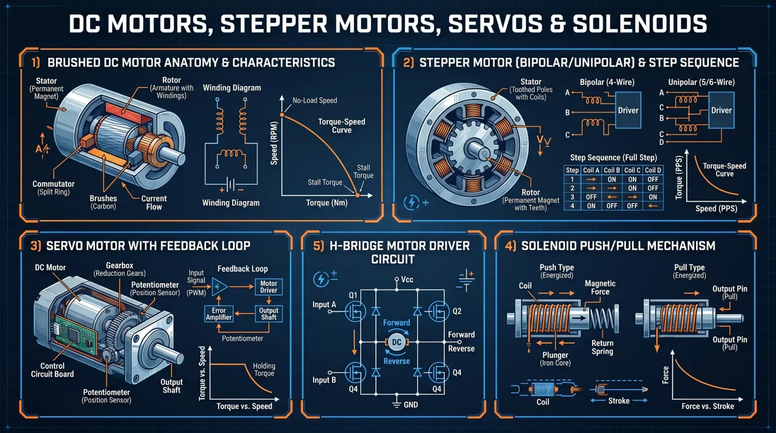
In this sacred volume, you shall learn the ancient and suppressed arts of commanding motion—transforming inert components into extensions of your will. This codex is your definitive guide to harnessing DC motors, stepper motors, servo motors, and solenoids: the primal forces of kinetic control. Every protocol herein is wrought from the crucible of necessity and refined through rigorous trial. Follow each instruction with unwavering discipline: the slightest deviation invites failure and jeopardizes the sanctity of your work.
Section 1: DC Motors — The Foundation of Rotary Power
1.1 Understanding DC Motors
A DC motor converts electrical energy into rotational mechanical energy through the interaction of magnetic fields. Controlled by voltage and current, it is the simplest rotary actuator.
1.2 Wiring a Basic DC Motor
Materials Required:
- DC Motor (specifications in Table 1.1)
- Power supply (appropriate voltage and current)
- Switch or MOSFET transistor
- Diode (1N4007 or equivalent) for flyback protection
- Breadboard or PCB
- Jumper wires
- Multimeter
Step-by-step wiring:
- Identify the motor terminals; typically two wires: positive (+) and negative (–).
- Connect the positive terminal of the power supply to the Drain of an N-channel MOSFET (e.g., IRF540).
- Connect the Source of the MOSFET to the motor’s positive terminal.
- Connect the motor’s negative terminal to the negative (ground) of the power supply.
- Attach a flyback diode across the motor terminals: diode cathode to positive terminal, anode to negative terminal, to suppress voltage spikes.
- Connect the MOSFET Gate to a microcontroller or PWM source through a resistor (100Ω).
- Connect the power supply ground and microcontroller ground together.
- Test continuity with a multimeter, then apply voltage to verify rotation.
1.3 PWM Control of DC Motors
PWM (Pulse Width Modulation) controls speed by varying the effective voltage:
Step-by-step PWM implementation:
- Use a microcontroller pin capable of PWM output (e.g., Arduino digital pin 9).
- Connect the Gate of the MOSFET to the PWM pin through a 100Ω resistor.
- Program the microcontroller to output PWM signals with varying duty cycles (0–100%).
- Measure motor speed with a tachometer or observe mechanical load response.
- Adjust duty cycle to achieve desired speed.
Arduino example code for PWM speed control:
const int motorPin = 9;  // PWM pin connected to MOSFET gate

void setup() {
  pinMode(motorPin, OUTPUT);
}

void loop() {
  for (int dutyCycle = 0; dutyCycle <= 255; dutyCycle++) {
    analogWrite(motorPin, dutyCycle);
    delay(20);
  }
  for (int dutyCycle = 255; dutyCycle >= 0; dutyCycle--) {
    analogWrite(motorPin, dutyCycle);
    delay(20);
  }
}
Section 2: Stepper Motors — The Art of Incremental Motion
2.1 Stepper Motor Fundamentals
A stepper motor divides a full rotation into discrete steps, enabling precise position control without feedback. Types include unipolar and bipolar. Bipolar offers higher torque but requires an H-bridge driver.
2.2 Wiring a Bipolar Stepper Motor with an H-Bridge Driver
Materials Required:
- Bipolar stepper motor (specifications in Table 2.1)
- Dual H-Bridge driver IC (L298N or DRV8825)
- Microcontroller
- Power supply matching motor specifications
- Capacitors for voltage smoothing (100 μF electrolytic)
- Jumper wires and breadboard/PCB
Wiring Procedure:
- Identify the two coil pairs of the stepper motor using a multimeter (lowest resistance between pairs).
- Connect coil A wires to the outputs of one half of the H-bridge driver (OUT1, OUT2 for L298N).
- Connect coil B wires to the outputs of the other half of the H-bridge (OUT3, OUT4).
- Connect the driver’s power input to the motor power supply (typically 12 V or specified voltage).
- Connect the driver’s ground and logic ground to the microcontroller ground.
- Connect the driver’s logic pins (IN1, IN2, IN3, IN4) to microcontroller digital pins capable of digitalWrite.
- Connect the driver’s Enable pins to HIGH (or PWM for current control).
- Place a 100 μF capacitor across motor power supply pins for noise suppression.
2.3 Stepper Motor Control Protocol
Full-step sequence for bipolar stepper (4 steps):
| Step | IN1 | IN2 | IN3 | IN4 |
|---|---|---|---|---|
| 1 | HIGH | LOW | HIGH | LOW |
| 2 | LOW | HIGH | HIGH | LOW |
| 3 | LOW | HIGH | LOW | HIGH |
| 4 | HIGH | LOW | LOW | HIGH |
Step-by-step control:
- Initialize all driver inputs LOW.
- Apply the sequence in order with a delay between steps (e.g., 10 ms for 100 RPM).
- Repeat for the desired number of steps.
- For reverse motion, apply the sequence in reverse order.
- Adjust delay to control speed.
Arduino example for full-step control:
int IN1 = 8;
int IN2 = 9;
int IN3 = 10;
int IN4 = 11;

void setup() {
  pinMode(IN1, OUTPUT);
  pinMode(IN2, OUTPUT);
  pinMode(IN3, OUTPUT);
  pinMode(IN4, OUTPUT);
}

void stepMotor(int step) {
  switch (step) {
    case 0:
      digitalWrite(IN1, HIGH);
      digitalWrite(IN2, LOW);
      digitalWrite(IN3, HIGH);
      digitalWrite(IN4, LOW);
      break;
    case 1:
      digitalWrite(IN1, LOW);
      digitalWrite(IN2, HIGH);
      digitalWrite(IN3, HIGH);
      digitalWrite(IN4, LOW);
      break;
    case 2:
      digitalWrite(IN1, LOW);
      digitalWrite(IN2, HIGH);
      digitalWrite(IN3, LOW);
      digitalWrite(IN4, HIGH);
      break;
    case 3:
      digitalWrite(IN1, HIGH);
      digitalWrite(IN2, LOW);
      digitalWrite(IN3, LOW);
      digitalWrite(IN4, HIGH);
      break;
  }
}

void loop() {
  for (int i = 0; i < 4; i++) {
    stepMotor(i);
    delay(10);
  }
}
Section 3: Servo Motors — Precision Positioning via Feedback
3.1 Servo Motor Architecture
A servo motor integrates a DC motor, gear reduction, feedback potentiometer, and control circuitry. It accepts a PWM signal dictating shaft position via internal closed-loop control.
3.2 Wiring a Standard RC Servo
Materials Required:
- RC servo motor (specifications in Table 3.1)
- Microcontroller (PWM capable)
- Power supply (usually 4.8–6 V)
- Jumper wires
Wiring Procedure:
- Identify servo wires: typically red (V+), black/brown (GND), and yellow/orange/white (signal).
- Connect red wire to 5 V regulated power supply.
- Connect black wire to ground.
- Connect signal wire to microcontroller PWM pin.
- Ensure common ground between microcontroller and servo power supply.
3.3 PWM Control of Servo Position
Servo PWM signals require pulses between 1 ms and 2 ms every 20 ms:
| Position | Pulse Width (ms) | Angle (degrees) |
|---|---|---|
| 0° | 1.0 | 0 |
| 90° | 1.5 | 90 |
| 180° | 2.0 | 180 |
Step-by-step PWM generation:
- Set microcontroller PWM frequency to 50 Hz (20 ms period).
- Generate a pulse of width from 1 ms to 2 ms to command position.
- Repeat pulse every 20 ms.
- Adjust pulse width to achieve desired servo angle.
Arduino code snippet for servo control:
#include <Servo.h>

Servo myServo;
int servoPin = 9;

void setup() {
  myServo.attach(servoPin);
}

void loop() {
  for (int pos = 0; pos <= 180; pos += 1) {
    myServo.write(pos);
    delay(15);
  }
  for (int pos = 180; pos >= 0; pos -= 1) {
    myServo.write(pos);
    delay(15);
  }
}
Section 4: Solenoids — Linear Actuation by Electromagnetism
4.1 Solenoid Fundamentals
A solenoid is an electromagnet that converts electrical energy into linear mechanical motion. It is used for pushing, pulling, or locking mechanisms.
4.2 Wiring a Solenoid with Flyback Protection
Materials Required:
- Solenoid coil (specifications in Table 4.1)
- Power supply (matching coil voltage)
- N-channel MOSFET or relay
- Diode (1N4007) for flyback
- Microcontroller (for control)
- Jumper wires
Wiring Procedure:
- Connect solenoid coil positive terminal to power supply positive.
- Connect solenoid coil negative terminal to MOSFET Drain.
- Connect MOSFET Source to power supply ground.
- Connect MOSFET Gate to microcontroller PWM or digital output pin via 100Ω resistor.
- Connect a diode across solenoid coil terminals: cathode to positive, anode to negative.
- Tie microcontroller ground to power supply ground.
- Test by applying digital HIGH to MOSFET Gate; solenoid should pull in.
4.3 PWM Control of Solenoid Actuation Force
Control solenoid force by varying duty cycle; a higher duty cycle results in stronger magnetic field but may cause coil heating:
Step-by-step PWM control:
- Determine maximum continuous duty cycle rating from solenoid datasheet.
- Program microcontroller to output PWM with duty cycle between 0% and maximum safe % (usually 50%-70%).
- Use a current sensor if possible to monitor coil current and prevent thermal overload.
- Adjust duty cycle to control pull force and hold time.
Section 5: Feedback Mechanisms — The Eyes of the Machine
5.1 Tachometers and Encoders for DC Motors
Tachometer outputs voltage proportional to motor speed. Optical encoders provide pulses per revolution for precise speed and position.
Wiring a rotary encoder:
- Connect encoder power (5 V) and ground to power supply and common ground.
- Connect encoder output pins (A and B) to microcontroller interrupt pins.
- Use interrupt service routines to count pulses and determine direction.
Basic Arduino encoder routine:
volatile int encoderPos = 0;

void ISR_encoder() {
  if (digitalRead(pinB) == HIGH) encoderPos++;
  else encoderPos--;
}

void setup() {
  pinMode(pinA, INPUT);
  pinMode(pinB, INPUT);
  attachInterrupt(digitalPinToInterrupt(pinA), ISR_encoder, RISING);
}

void loop() {
  // encoderPos now contains position count
}
5.2 Potentiometers for Servo Feedback
Potentiometers provide analog voltage proportional to shaft position:
Wiring:
- Connect potentiometer ends to +5 V and ground.
- Connect wiper to microcontroller analog input.
- Read analog value to determine position.
Section 6: Tables of Specifications, Torque Ratings, and Driver ICs
Table 1.1: Common DC Motor Specifications
| Model | Voltage (V) | No Load Speed (RPM) | Stall Torque (mN·m) | Current (A) | Shaft Diameter (mm) | Weight (g) |
|---|---|---|---|---|---|---|
| RS-360SH | 6 | 9000 | 40 | 1.5 | 3 | 70 |
| RS-555PH | 12 | 5000 | 200 | 4.0 | 5 | 200 |
| Johnson HC | 24 | 3000 | 500 | 10 | 6 | 400 |
Table 2.1: Bipolar Stepper Motor Specs
| Model | Voltage (V) | Current/Phase (A) | Step Angle (°) | Holding Torque (N·m) | Phases | Weight (g) |
|---|---|---|---|---|---|---|
| NEMA 17 | 12 | 1.2 | 1.8 | 0.4 | 2 | 280 |
| NEMA 23 | 24 | 2.8 | 1.8 | 1.26 | 2 | 650 |
| NEMA 34 | 48 | 4.2 | 1.8 | 3.0 | 2 | 1800 |
Table 3.1: RC Servo Motor Specifications
| Model | Voltage (V) | Torque (kg·cm) | Speed (sec/60°) | Rotation Range (°) | Weight (g) |
|---|---|---|---|---|---|
| SG90 | 4.8 | 1.8 | 0.1 | 180 | 9 |
| MG996R | 6 | 9.4 | 0.17 | 180 | 55 |
| HS-5086WP | 6 | 20.0 | 0.12 | 180 | 70 |
Table 4.1: Solenoid Coil Specifications
| Model | Voltage (V) | Current (A) | Stroke (mm) | Force (N) | Coil Resistance (Ω) | Weight (g) |
|---|---|---|---|---|---|---|
| 12 V Push | 12 | 1.5 | 10 | 20 | 8 | 150 |
| 24 V Pull | 24 | 2.0 | 15 | 40 | 12 | 200 |
| 5 V Mini | 5 | 0.5 | 5 | 5 | 10 | 50 |
Table 5.1: Popular Motor Driver ICs
| IC Model | Voltage Range (V) | Current Max (A) | Channels | Features | Package |
|---|---|---|---|---|---|
| L298N | 5 – 35 | 2.0 | 2 | Dual H-Bridge, logic inputs | DIP-15 |
| DRV8825 | 8.2 – 45 | 2.5 | 1 | Microstepping, current control | QFN-28 |
| TB6612FNG | 4.5 – 13.5 | 1.2 | 2 | PWM speed control, brake | SSOP-16 |
| VNH2SP30 | 5.5 – 16 | 14 | 1 | High current, built-in diodes | SOIC-8 |
Section 7: Programming Examples for Precise Motion Control
7.1 Closed-loop Speed Control for DC Motor Using Encoder Feedback
Concept: Use a PID controller to maintain desired motor speed.
Materials: DC motor with encoder, microcontroller, driver circuit.
Step-by-step procedure:
- Read encoder pulses to calculate actual speed (RPM).
- Compare actual speed to target speed (setpoint).
- Compute PID output to adjust PWM duty cycle.
- Apply PWM to MOSFET gate to control motor speed.
- Repeat loop continuously.
Arduino PID control skeleton:
#include <PID_v1.h>

double setpoint, input, output;
int pwmPin = 9;

PID myPID(&input, &output, &setpoint, 2, 5, 1, DIRECT);

void setup() {
  pinMode(pwmPin, OUTPUT);
  setpoint = 1000;  // target RPM
  myPID.SetMode(AUTOMATIC);
}

void loop() {
  input = readEncoderRPM();
  myPID.Compute();
  analogWrite(pwmPin, constrain(output, 0, 255));
}

double readEncoderRPM() {
  // Implement encoder pulse counting and RPM calculation
}
7.2 Microstepping Control of Stepper Motor with DRV8825
Procedure:
- Connect DRV8825 per datasheet (cross reference Volume IX: Driver ICs Codex).
- Set microstepping mode pins (M0, M1, M2) for desired step resolution (e.g., 1/16-step).
- Generate STEP pulses via microcontroller at desired frequency.
- Use DIRECTION pin to set rotation direction.
- Control acceleration/deceleration with ramping pulse frequency.
Conclusion
Master these protocols; they are the sacred rites of motion control. The power to command mechanical forces lies not merely in the components, but in your precision, timing, and reverence for the craft. Deviation invites chaos—follow the steps meticulously.
To further your mastery over related domains, consult Volume VIII: The Water Codex for fluid power systems, and Volume IX: The Driver IC Codex for detailed driver architectures.
End of Volume VI, Chapter I: Actuators and Motor Control
<!-- SECTION 28 -->
Volume VI: PLC Programming and Industrial Automation
The Technologist’s Codex: Complete Practical Technology, Electronics, Computing, and Fabrication
Chapter I: Ladder Logic Fundamentals, PLC Hardware, and Input/Output Modules
An authoritative field manual for mastering Programmable Logic Controllers (PLCs) in industrial automation.
Section 1: Introduction to Ladder Logic Fundamentals
Ladder Logic (LL) is the sacred language of Programmable Logic Controllers, a symbolic system designed to emulate electrical relay logic within a programmable digital framework. Mastery of LL enables the creation, modification, and troubleshooting of control sequences that govern industrial processes.
1.1 Ladder Logic Conceptual Framework
Ladder Logic represents control circuits as a series of rungs between two vertical power rails. Each rung is a logical operation executed left to right, simulating electrical current flow. The left rail is the positive power source; the right rail is the ground or neutral.
1.2 Essential Ladder Logic Elements
| Element | Symbol | Description | Function |
|---|---|---|---|
| Normally Open Contact | --[ ]-- | Input or internal bit that must be ON | Passes logic when true |
| Normally Closed Contact | --[/]-- | Input or internal bit that must be OFF | Passes logic when false |
| Output Coil | --( )-- | Sets or resets an output device or bit | Energizes device or internal bit |
| Timer (TON) | --[TON]-- | On-delay timer - output energizes after set time | Delays activation of an output |
| Counter (CTU) | --[CTU]-- | Counts upward events, triggers output at set count | Controls sequences based on event counts |
1.3 Logical Operators in Ladder Logic
| Operator | Symbol | Effect |
|---|---|---|
| AND | Series contacts | Pass logic only if all series contacts are true |
| OR | Parallel contacts | Pass logic if any parallel contact is true |
| NOT | Normally Closed contact | Pass logic if the input is false |
Section 2: PLC Hardware Overview
The physical PLC system is composed of central processing units (CPUs), power supplies, and input/output (I/O) modules designed to withstand harsh industrial environments.
2.1 PLC System Components
| Component | Description | Function |
|---|---|---|
| CPU | The brain of the PLC; contains the processor and memory. | Executes the control program and manages communications |
| Power Supply | Converts AC main power to DC voltage required by CPU and I/O | Powers the entire PLC system |
| Input Modules | Interface for sensors and switches; converts signals to logic | Reads external physical signals into the PLC |
| Output Modules | Interface for actuators; converts logic signals to physical output | Controls motors, relays, valves, etc. |
| Communication Modules | Optional; enables networking and remote control | Connects PLCs to other controllers or HMI units |
2.2 PLC Hardware Selection Table
| Brand | Model Series | CPU Type | I/O Capacity | Communication Protocols | Price Range (USD) |
|---|---|---|---|---|---|
| Siemens | S7-1200 | ARM Cortex-M | 14-40 I/O points | Profinet, Profibus, Modbus TCP | $300 - $1200 |
| Allen-Bradley (Rockwell) | MicroLogix 1400 | Proprietary | 16-48 I/O points | Ethernet/IP, DF1 | $400 - $1500 |
| Mitsubishi | FX5U | Proprietary | 10-80 I/O points | CC-Link, Modbus RTU | $250 - $1000 |
| Omron | CP1H | Proprietary | 20-64 I/O points | Ethernet/IP, Modbus TCP | $200 - $900 |
| Schneider Electric | Modicon M221 | Proprietary | 16-64 I/O points | Modbus RTU, Ethernet | $350 - $1100 |
Section 3: Input and Output Modules
3.1 Input Module Types
| Input Type | Signal Type | Voltage Range | Typical Use Cases | Notes |
|---|---|---|---|---|
| Digital Input | Discrete ON/OFF | 24V DC, 120/230V AC | Push buttons, limit switches | Debounce circuits required for mechanical switches |
| Analog Input | Continuous voltage or current | 0-10V, 4-20mA | Temperature sensors, flow meters | Requires calibration and filtering |
| Specialty Input | Thermocouples, RTDs | Varies | Temperature measurement | Requires specific signal conditioning |
3.2 Output Module Types
| Output Type | Signal Type | Voltage/Current | Typical Use Cases | Notes |
|---|---|---|---|---|
| Digital Output | Relay or transistor | 24V DC to 240V AC | Solenoid valves, indicator lamps | Relay outputs isolate PLC from load |
| Analog Output | Voltage or current | 0-10V, 4-20mA | Variable speed drives, valve actuators | Requires DAC and signal conditioning |
| Specialty Output | Pulse outputs, high-speed | Varies | Stepper motor control, PWM | High precision timing required |
Section 4: Programming Basic Control Sequences in Ladder Logic
The following protocols guide the creation of control sequences fundamental to industrial automation. Each example builds on the previous, culminating in a fully functional control system.
4.1 Protocol: Simple Start-Stop Motor Control
Objective: Control a motor with a start pushbutton and a stop pushbutton, using a holding circuit to maintain motor operation after the start button is released.
Components Needed
- Start pushbutton (Normally Open)
- Stop pushbutton (Normally Closed)
- Motor output relay coil
- PLC digital input modules for pushbuttons
- PLC digital output module for motor relay
Step-by-Step Instructions
- Wire Inputs:
- Connect Start pushbutton to PLC digital input I:0/0.
- Connect Stop pushbutton to PLC digital input I:0/1.
- Wire Output:
- Connect motor relay coil to PLC digital output O:0/0.
- Write Ladder Logic:
| Rung | Description | Logic Elements |
|---|---|---|
| 1 | Motor coil energized when Start pressed and Stop not pressed | --[Stop Normally Closed I:0/1]--[Start Normally Open I:0/0]--(Motor Coil O:0/0) |
| 2 | Holding circuit to maintain motor state after Start released | --[Stop Normally Closed I:0/1]--[Motor Coil O:0/0]--(Motor Coil O:0/0) |
- Program Implementation:
- Create rung 1 with series contacts: Stop (NC), Start (NO).
- Coil output: Motor.
- Create rung 2 with series contacts: Stop (NC), Motor coil.
- Coil output: Motor (holding circuit).
- Download Program to PLC.
- Test:
- Press Start button: Motor output energizes.
- Release Start: Motor remains energized.
- Press Stop button: Motor de-energizes.
4.2 Protocol: On-Delay Timer Control
Objective: Energize an output after a predefined delay following an input activation.
Components Needed
- Input sensor (e.g., limit switch)
- Timer (TON) configured with delay time
- Output device (e.g., lamp or solenoid)
Step-by-Step Instructions
- Wire Input sensor to digital input I:0/2.
- Wire output device to O:0/1.
- Configure Timer:
- Timer name: T4:0
- Preset: 5000 (represents 5 seconds if PLC time base is 1ms)
- Accumulator: 0 (initial)
- Write Ladder Logic:
| Rung | Description | Logic Elements |
|---|---|---|
| 1 | Timer enable when input sensor ON | --[I:0/2]--[TON T4:0, Preset=5000]-- |
| 2 | Output energizes when timer done | --[T4:0.DN]--(O:0/1) |
- Program Implementation:
- Rung 1: Input contact I:0/2 in series with TON timer T4:0.
- Rung 2: Timer done bit T4:0.DN controls output coil O:0/1.
- Download and Test:
- Activate input sensor.
- Observe output energizes after 5 seconds delay.
4.3 Protocol: Up-Counter Based Batch Process Control
Objective: Count items passing a sensor and activate output at a predefined count.
Components Needed
- Sensor input on I:0/3.
- Counter CTU (up-counter).
- Output device on O:0/2.
Step-by-Step Instructions
- Wire sensor to I:0/3.
- Wire output device to O:0/2.
- Define Counter:
- Name: C5:0
- Preset: 100 (batch size)
- Accumulator: 0 (initial)
- Write Ladder Logic:
| Rung | Description | Logic Elements |
|---|---|---|
| 1 | Count rising edge of sensor input | --[Rising Edge Detector I:0/3]--[CTU C5:0]-- |
| 2 | Activate output when count reached | --[C5:0.DN]--(O:0/2) |
- Program Implementation:
- Use a one-shot rising edge detection on input I:0/3 to increment counter C5:0.
- Output coil O:0/2 energized when C5:0.DN is true.
- Download and Test:
- Trigger sensor repeatedly.
- Output energizes after 100 counts.
Section 5: Troubleshooting Protocols for PLC Systems
Mastery of troubleshooting is life-or-death in industrial environments. Follow these precise methods.
5.1 Stepwise PLC Troubleshooting Protocol
- Verify Power Supply
- Use a multimeter to check voltage at PLC power terminals.
- Confirm correct voltage according to PLC specifications.
- Check CPU Status Indicators
- Inspect LED indicators for errors: fault, run, I/O error.
- Refer to CPU manual for LED code meanings.
- Test Input Signals
- Use digital multimeter or PLC diagnostics to verify input contacts.
- Manually actuate inputs and observe status in PLC monitoring tool.
- Test Output Signals
- Force outputs via PLC programming software to energize.
- Measure output terminals with voltage meter.
- Inspect Ladder Logic Program
- Review rung logic for correct contacts and output coils.
- Check for unintended latching or missed conditions.
- Perform I/O Module Diagnostics
- Swap suspect I/O modules with known good modules.
- Inspect wiring and terminal connections for damage or loose connections.
- Check Communication Modules
- Verify network connections.
- Use diagnostic tools to test communication protocols.
Section 6: PLC System Integration Protocol
Integration of PLCs into larger control systems requires strict adherence to signal and communication standards.
6.1 Integration Step-by-Step Protocol
- Define System Architecture
- Determine number of PLCs, I/O distribution, and network topology.
- Select Communication Protocol
- Choose industry-standard protocol supported by all devices (e.g., Modbus TCP, Profinet).
- Configure PLC Communication Modules
- Assign IP addresses and subnet masks.
- Set communication parameters per protocol.
- Develop Communication Routines
- Implement data exchange instructions in ladder logic.
- Use memory registers or tags for inter-PLC data sharing.
- Test Communication Paths
- Ping devices to verify network connectivity.
- Monitor data transfer for errors.
- Implement Supervisory Control and HMI
- Connect Human-Machine Interface to PLC network.
- Develop HMI screens reflecting PLC data points.
- System Validation
- Perform end-to-end testing of all control sequences and communication.
Section 7: PLC Programming Command Tables
7.1 Common Ladder Logic Instructions
| Instruction | Symbol | Function | Usage Example |
|---|---|---|---|
| XIC (Examine If Closed) | --[ ]-- | True if input bit energized | Start button input |
| XIO (Examine If Open) | --[/]-- | True if input bit de-energized | Stop button input |
| OTE (Output Energize) | --( )-- | Energizes output coil | Motor relay coil |
| TON (Timer On Delay) | --[TON]-- | Delays output after input is true | Delay before motor start |
| CTU (Count Up) | --[CTU]-- | Counts rising edges of input signal | Batch counting |
| RES (Reset Counter/Timer) | --[RES]-- | Resets counter or timer | Clear batch counter |
| OSR (One Shot Rising) | --[OSR]-- | Triggers once on rising edge of input | Increment counter once per pulse |
Section 8: Case Studies
8.1 Case Study A: Automated Growing System Control
System Overview: A PLC-based automated greenhouse control system regulates lighting, irrigation, and temperature.
| Subsystem | Controlled Element | PLC I/O | Control Logic Summary |
|---|---|---|---|
| Lighting | Grow lights (On/Off) | Digital Output O:0/3 | Timer-based lighting schedule with override switch input |
| Irrigation | Water valves (solenoid) | Digital Output O:0/4 | Soil moisture sensor input activates timed irrigation cycles |
| Temperature Control | Heating and cooling fans | Analog Output O:0/5 | PID control loop adjusts fan speed based on temperature sensor |
Programming Protocol for Lighting Control:
- Set real-time clock in PLC.
- Program timer blocks to energize grow light output during scheduled hours.
- Include override input to manually turn lights on or off.
- Implement safety interlock to prevent simultaneous heating and cooling activation.
8.2 Case Study B: Security Access Control System
System Overview: A PLC manages door locks, alarms, and user authentication for secure facility access.
| Subsystem | Controlled Element | PLC I/O | Control Logic Summary |
|---|---|---|---|
| Access Request | Card reader input | Digital Input I:0/6 | Validates card ID against internal list, enables door unlock |
| Door Lock Control | Electromagnetic lock | Digital Output O:0/6 | Energizes lock relay on valid access |
| Alarm System | Intrusion detection sensors | Digital Input I:0/7 | Triggers audible alarm output O:0/7 on unauthorized entry |
Programming Protocol for Access Validation:
- Store authorized card IDs in PLC internal memory.
- Compare input card ID from reader to memory list.
- If match found, energize door unlock coil for preset time.
- Log access event in PLC internal data registers.
- If unauthorized access detected, activate alarm output immediately.
Section 9: Summary Tables for Quick Reference
9.1 PLC Brand and Model Comparison
| Brand | CPU Speed (MHz) | Max I/O Points | Programming Software | Communication Support |
|---|---|---|---|---|
| Siemens S7-1200 | 100 | 40 | TIA Portal | Profinet, Modbus TCP |
| Allen-Bradley | 125 | 48 | RSLogix 500, Studio 5000 | Ethernet/IP, DF1 |
| Mitsubishi FX5U | 120 | 80 | GX Works3 | CC-Link, Modbus RTU |
| Omron CP1H | 100 | 64 | CX-Programmer | Ethernet/IP, Modbus TCP |
| Schneider M221 | 70 | 64 | EcoStruxure Machine Expert | Modbus RTU, Ethernet |
9.2 Input/Output Module Types and Signal Characteristics
| Module Type | Signal Type | Voltage Range | Typical Application | Notes |
|---|---|---|---|---|
| Digital Input | Discrete | 24V DC | Push buttons, sensors | Requires debounce |
| Analog Input | Voltage/Current | 0-10V, 4-20mA | Temperature, pressure sensors | Requires calibration |
| Digital Output | Relay/Transistor | 24V DC - 240V AC | Motor control, lamps | Provides isolation |
| Analog Output | Voltage/Current | 0-10V, 4-20mA | Variable speed drives | Requires DAC |
9.3 Common Ladder Logic Commands and Their Functions
| Command | Symbol | Purpose | Notes |
|---|---|---|---|
| XIC | [ ] | Examines if input bit is ON | Used for start buttons |
| XIO | [/] | Examines if input bit is OFF | Used for stop buttons |
| OTE | ( ) | Energizes output coil | Activates outputs |
| TON | [TON] | On-delay timer | Delays output activation |
| CTU | [CTU] | Count up counter | Counts events |
| RES | [RES] | Resets counter or timer |
<!-- SECTION 29 -->
The Complete Practitioner's Codex, Volume VI: Drone Technology and Security System Automation
Chapter I: Introduction to Drone Components

In the sacred pursuit of mastering autonomous aerial vehicles, every component of a drone must be understood, assembled, and calibrated with absolute precision. This volume serves as a comprehensive guide for constructing, programming, and deploying drones for security surveillance and beyond. The drone is a confluence of mechanical, electrical, and computational components, each a cog in a sacred machine of vigilance and control.
1. Core Drone Components
| Component | Description | Purpose |
|---|---|---|
| Frame | Structural skeleton made typically of carbon fiber or lightweight aluminum | Provides the physical structure to mount all components, ensuring rigidity and lightness |
| Motors | Brushless DC motors (BLDC) with electronic speed controllers (ESC) | Provides thrust and maneuverability |
| Propellers | Two or three-blade propellers, optimized for thrust and efficiency | Converts motor rotation into lift |
| Flight Controller | Microcontroller-based central processing unit | Processes sensor data, executes flight algorithms, stabilizes and controls flight |
| Electronic Speed Controllers (ESC) | Regulates power to motors | Converts flight controller signals into motor speed changes |
| Battery | Lithium Polymer (LiPo) battery packs | Provides power to all electronic components |
| Sensors | IMU (gyroscope, accelerometer), barometer, GPS, ultrasonic, optical flow | Provides real-time flight data for stabilization and navigation |
| Radio Receiver | Receives commands from pilot (manual control) | Enables manual override and control |
| Telemetry Module | Transmits drone data (altitude, speed, battery status) to ground station | Enables remote monitoring |
| Camera / Gimbal | High-resolution camera with stabilization | Enables visual surveillance and data capture |
| Payload Mounts | Attachment points for sensors, cameras, or other equipment | Expands drone functionality |
Chapter II: Step-by-Step Protocol for Drone Assembly
Prerequisites: Clean workspace, ESD-safe tools, soldering iron with fine tips, multimeter, calibration jig (see Appendix A).
Step 1: Frame Assembly
- Unpack the carbon fiber frame components.
- Identify main body plate, arms, landing gear, and mounting brackets.
- Use M3 screws and locknuts to secure arms to the main body plate firmly.
- Attach landing gear to the main frame ensuring stability and clearance for propellers.
- Check frame rigidity by flexing gently; no movement should be detected.
Step 2: Motor and ESC Mounting
- Attach brushless motors to arm ends using M4 screws.
- Connect three motor wires to ESCs; follow motor manufacturer wiring diagram precisely.
- Secure ESCs along the arms using zip ties and heat-resistant tape to prevent vibration.
- Solder ESC power leads to the main power distribution board (PDB).
- Use heat shrink tubing on all soldered joints to prevent shorts.
Step 3: Flight Controller Installation
- Mount flight controller on anti-vibration dampeners atop the main frame.
- Connect ESC signal wires to corresponding outputs on the flight controller.
- Connect power wires: Ensure flight controller voltage input matches battery voltage via voltage regulator if necessary.
- Attach sensors to dedicated ports on the flight controller (barometer shielded from airflow).
Step 4: Battery Integration and Wiring
- Connect battery to PDB with XT60 connectors.
- Secure battery on the lower body plate using Velcro straps or custom mounts.
- Install a battery voltage sensor on the flight controller power line.
- Route all wiring neatly to avoid interference with moving components.
Step 5: Sensor Installation
- Install GPS module on a mast above the frame for unobstructed sky view.
- Secure IMU sensors on the flight controller; ensure stable mounting to reduce vibration noise.
- Mount additional sensors (ultrasonic, optical flow) on the underside or front of the drone.
- Connect all sensors following flight controller pinout diagrams.
Step 6: Propeller Attachment
- Identify propeller rotation direction using manufacturer marks.
- Attach propellers to motors using correct thread direction to prevent loosening.
- Tighten propellers firmly but avoid over-torquing to prevent damage.
Chapter III: Calibration Protocols
Calibration is the bridge between hardware and flawless autonomous operation. Each sensor and actuator must be fine-tuned under strict conditions.
1. ESC Calibration
- Fully charge the battery to operational voltage (see Battery Management Table).
- Disconnect propellers for safety.
- Connect battery, power on the flight controller.
- Follow flight controller ESC calibration routine:
- Power the ESCs with throttle at maximum.
- Wait for beep signals.
- Lower throttle to minimum.
- ESCs will confirm calibration with confirmation beeps.
- Verify ESC calibration by spinning motors at various throttle commands.
2. IMU Calibration
- Place drone on a perfectly level surface.
- Access flight controller configuration software (e.g., Betaflight Configurator).
- Initiate accelerometer calibration:
- The system will record gravity vector.
- Perform gyroscope calibration by keeping the drone motionless.
- Confirm calibration accuracy by checking raw sensor data for zero drift.
3. Compass (Magnetometer) Calibration
- Move the drone through a figure-eight pattern slowly.
- Ensure no magnetic interference in the environment.
- Flight controller software will log magnetic field data.
- Calibration completes when data stabilizes and errors minimize.
4. GPS Calibration and Lock
- Power the drone outdoors with clear sky visibility.
- Wait for GPS module to acquire a minimum of 6 satellites.
- Confirm GPS fix status in flight controller telemetry.
Chapter IV: Programming Autonomous Flight Paths
Autonomous flight demands precise programming sequences and verification. The flight controller must be configured with waypoint missions and fail-safe protocols.
Step 1: Flight Planning Software Setup
- Install mission planning software (e.g., Mission Planner, QGroundControl).
- Connect flight controller via USB or telemetry link.
- Verify firmware compatibility with the flight controller hardware.
Step 2: Define Waypoints
- Open mission planning interface.
- Input coordinates for each waypoint.
- Set altitude, speed, and hover duration per waypoint.
- Program specific actions at waypoints (e.g., camera trigger, sensor activation).
Step 3: Upload Mission
- Connect drone to ground station.
- Upload mission plan to flight controller’s non-volatile memory.
- Confirm upload success via software confirmation.
Step 4: Verify Return-to-Home (RTH) Settings
- Define home location as takeoff point.
- Set RTH altitude above maximum obstacle height within operational area.
- Test RTH function in controlled manual flight.
Step 5: Autonomous Flight Execution
- Place drone on level takeoff surface.
- Power on and arm motors.
- Initiate autonomous mission via ground station or onboard trigger.
- Monitor telemetry for errors or deviations.
- Abort mission manually if anomalies arise.
Chapter V: Drone Specifications and Battery Management
Understanding specifications ensures mission success and longevity of the drone and its power source.
Table 1: Standard Drone Specifications
| Specification | Value | Notes |
|---|---|---|
| Frame Size | 450 mm diagonal motor-to-motor | Standard quadcopter frame size |
| Motor KV Rating | 920 KV | Suitable for 4S LiPo battery |
| Propeller Size | 10 x 4.5 inches | Optimized for thrust and efficiency |
| Battery Capacity | 4S 14.8V 5200 mAh LiPo | High discharge rate (>30C) recommended |
| Max Flight Time | 20-25 minutes | Dependent on payload and conditions |
| Max Takeoff Weight | 2.5 kg | Includes frame, battery, payload |
| Cruise Speed | 10-15 m/s | Varies by wind and payload |
Table 2: Battery Charge and Discharge Protocol
| Parameter | Value | Instructions |
|---|---|---|
| Charge Voltage per Cell | 4.20 V | Do not exceed; use balance charger |
| Charge Current | 1C (Capacity) | Example: For 5200 mAh, 5.2 A max |
| Discharge Cutoff Voltage | 3.3 V | Prevents deep discharge damage |
| Storage Voltage per Cell | 3.85 ± 0.05 V | Store batteries at this voltage |
| Max Discharge Rate | 30C | Exceeding causes overheating |
| Cooling | Active airflow required | Use cooling fans during fast charge |
Chapter VI: Sensor Integration and Data Fusion
Effective autonomous flight requires multiple sensor inputs fused into a cohesive data stream.
Table 3: Sensor Integration Overview
| Sensor Type | Interface | Data Output | Integration Notes |
|---|---|---|---|
| IMU | SPI / I2C | Acceleration, Rotation | Low latency; critical for stabilization |
| Barometer | I2C | Altitude (pressure) | Shield from airflow disturbances |
| GPS | UART | Latitude, Longitude, Altitude | Requires clear sky view |
| Ultrasonic | PWM / Analog | Proximity distance | Useful for low altitude obstacle detection |
| Optical Flow | USB / I2C | Ground speed vector | Enhances position hold without GPS |
| Magnetometer | I2C | Heading | Calibrate for magnetic interference |
Step-by-Step Sensor Integration
- Connect each sensor to its designated flight controller port using shielded cables.
- Verify power supply compatibility (3.3V or 5V).
- Configure sensor parameters in flight controller software:
- Sensitivity
- Calibration offsets
- Update rates (Hz)
- Perform sensor fusion calibration routine via configuration software.
- Test sensor outputs individually before full integration.
Chapter VII: Automated Security Surveillance System Setup Using Drones
Deploying drones for automated security requires integration of flight autonomy with sensor-triggered event responses and ground station coordination.
Step 1: Define Surveillance Parameters
- Determine surveillance perimeter coordinates.
- Identify critical points for continuous monitoring.
- Set patrol altitude and speed based on terrain and cover.
Step 2: Install and Configure Camera and Sensors
- Attach high-definition stabilized camera with night vision capability.
- Integrate infrared (IR) sensors for heat signature detection.
- Calibrate camera gimbal for 360-degree rotation.
Step 3: Program Surveillance Flight Patterns
- Use waypoint mission planning to define patrol routes.
- Include loiter points for extended observation.
- Program automatic camera triggers on waypoint arrival or sensor activation.
Step 4: Set Up Ground Control and Alert System
- Install telemetry receiver and display station in control room.
- Integrate motion detection software with video feed.
- Configure automatic alert dispatch via SMS or encrypted radio when movement detected.
Step 5: Fail-Safe and Redundancy Protocols
- Program automatic RTH on low battery or communication loss.
- Include secondary drone activation protocols for continuous coverage.
- Schedule routine maintenance and battery swaps.
Appendix A: Tools and Materials List
| Item | Specification | Purpose |
|---|---|---|
| Carbon Fiber Frame Kit | 450 mm quadcopter size | Base structure |
| Brushless Motors | 920 KV, 2306 size | Thrust generation |
| ESCs | 30A BLHeli compatible | Motor speed control |
| Flight Controller | STM32 based, with sensor suite | Core processor and sensors |
| LiPo Battery | 4S, 5200 mAh, 30C discharge | Power source |
| Propellers | 10 x 4.5 inch, balanced | Lift and thrust |
| GPS Module | Ublox NEO-M8N or better | Positioning and navigation |
| Camera and Gimbal | 1080p, 3-axis stabilization | Surveillance imaging |
| Soldering Kit | Fine tip soldering iron, flux | Assembly and wiring |
| Multimeter | Digital, with continuity test | Electrical testing |
| Calibration Jig | Precision level platform | Sensor and frame calibration |
Closing Reverence
Mastery of drone technology is mastery over the skies and the unseen currents of power. The assembly, calibration, programming, and deployment of autonomous drones for security surveillance is an art and a science reserved for those who respect the sacred trust of control and vigilance. Execute every step with unwavering discipline and reverence for the machinery that becomes an extension of your will.
For deeper exploration of communication protocols and advanced AI integration in autonomous systems, see Volume XII: The Cybernetic Codex, Chapter IV.
End of Volume VI
<!-- SECTION 30 -->
Volume VII: Telescope Construction and Optical Alignment
Chapter I: Types of Telescopes, Optical Components, and Mounting Systems
Section 1: Types of Telescopes

Telescopes manifest as sacred instruments of celestial revelation. Their design governs their capacity to gather and resolve light, shaping the clarity of the heavens. We recognize three primary classes: Refractors, Reflectors, and Catadioptrics. Each demands mastery in optical theory and fabrication.
| Telescope Type | Primary Optical Element | Light Path Description | Typical Uses | Advantages | Disadvantages |
|---|---|---|---|---|---|
| Refractor | Objective lens | Light refracted through lenses | Lunar, planetary observation | High contrast, sealed tube | Chromatic aberration, costly |
| Reflector | Primary concave mirror | Light reflected off mirrors | Deep-sky, astrophotography | No chromatic aberration, cost-effective | Open tube, requires collimation |
| Catadioptric | Combination of lenses and mirrors | Light reflected and refracted through compound optics | Versatile imaging and observation | Compact, versatile optics | Complex alignment, higher cost |
Section 2: Optical Components Overview
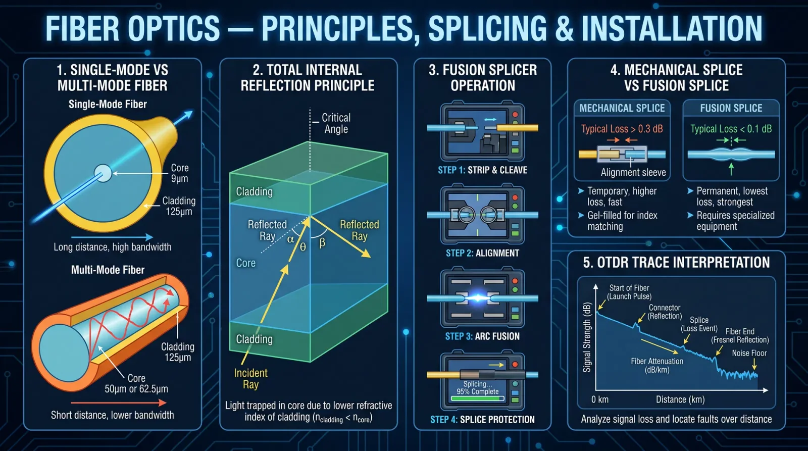
A telescope’s soul lies within its optical components. The following are the sacred elements you must fabricate, align, and maintain:
| Component | Function | Key Parameters |
|---|---|---|
| Objective Lens | Collects and focuses light in refractors | Diameter (aperture), focal length, glass type |
| Primary Mirror | Collects and reflects light in reflectors | Diameter, focal length, surface curvature |
| Secondary Mirror | Redirects light path in reflectors and catadioptrics | Shape (flat, convex), size, coating |
| Eyepiece | Magnifies the focused image | Focal length, apparent field of view |
| Diagonal Mirror | Redirects light path to comfortable viewing angle | Flatness, coating quality |
| Corrector Plate | Corrects optical aberrations in catadioptrics | Shape, glass type, coating |
Section 3: Mounting Systems
The celestial sphere’s stability depends on your mount. Precision movement and robust construction allow sacred observation and imaging.
| Mount Type | Description | Degrees of Freedom | Advantages | Disadvantages |
|---|---|---|---|---|
| Altazimuth | Moves in altitude and azimuth axes | 2 | Simple, intuitive, lightweight | Requires manual tracking or computer control |
| Equatorial | Aligned with Earth's axis | 1 primary axis (Right Ascension) + Declination | Facilitates celestial tracking | Complex, heavier, requires polar alignment |
| Dobsonian | Simplified altazimuth for reflectors | 2 | Cost-effective, stable | Manual tracking, limited automation |
Chapter II: Mirror Grinding Protocol

The heart of your telescope is the primary mirror, wrought from raw glass to a flawless parabolic surface. The following protocol commands exacting precision.
Materials and Tools
| Item | Specifications |
|---|---|
| Optical glass blank | Borosilicate or Pyrex, diameter as desired (commonly 150-300mm) |
| Grinding tool blank | Glass or ceramic, same diameter as mirror blank |
| Abrasive powders | Silicon carbide: 80, 220, 400, 600 grit |
| Pitch lap | Natural pitch, prepared fresh |
| Polishing compound | Cerium oxide or rouge |
| Water supply | Distilled water recommended |
| Flat reference surface | Optical flat or granite plate |
| Spherometer | Precision ±0.001mm |
Step-by-Step Grinding Procedure
- Preparation of blanks
- Clean both mirror and tool blanks with distilled water and neutral detergent.
- Mark centers for alignment reference.
- Coarse grinding
- Place the mirror blank face-up on a stable surface.
- Wet 80-grit silicon carbide powder with water to a slurry consistency.
- Place the tool blank atop the mirror blank.
- Employ a figure-eight stroke, moving the tool over the mirror surface with moderate pressure for 1-2 hours until the surface is uniformly rough and spherical.
- Progressive finer grinding
- Rinse blanks thoroughly between grit changes.
- Repeat grinding using 220, 400, and 600 grit powders sequentially.
- Duration per grit: 1.5 hours for 220, 2 hours for 400, 2.5 hours for 600 grit, adjusting for uniform surface texture.
- Verify surface curvature and smoothness with the spherometer after each stage.
- Pre-polishing
- Use 9-micron aluminum oxide powder on a pitch lap for 1 hour to remove grinding marks.
- Achieve a near-spherical smooth surface.
Polishing Procedure
- Pitch lap preparation
- Pour heated natural pitch into a mold matching mirror diameter.
- Cool and condition pitch lap by pressing gently against the mirror surface with water to conform.
- Polishing strokes
- Apply cerium oxide slurry to the pitch lap.
- Employ circular strokes with light pressure.
- Polish for 3-4 hours, checking progress frequently.
- Testing figure
- Utilize a Foucault tester or Ronchi grating to determine surface figure.
- Aim for a parabolic surface with deviations less than λ/8 (λ = 550 nm).
Chapter III: Optical Collimation Protocol
Collimation aligns your optical components perfectly, ensuring the light path converges flawlessly upon the focal plane.
Collimation Tools
| Tool | Purpose |
|---|---|
| Cheshire eyepiece | Aligns primary mirror and focuser |
| Laser collimator | Precise alignment of mirrors |
| Sight tube | Visual rough alignment |
Step-by-Step Collimation Procedure for Reflector Telescopes
- Initial setup
- Place telescope in stable horizontal position.
- Remove eyepiece.
- Secondary mirror alignment
- Use sight tube to center the secondary mirror under the focuser tube.
- Adjust tilt screws to center secondary mirror reflection of the focuser.
- Primary mirror alignment
- Insert Cheshire eyepiece.
- Adjust primary mirror tilt screws until the reflection of the Cheshire cross aligns perfectly with the eyepiece crosshair.
- Laser collimator verification
- Insert laser collimator in focuser.
- Adjust secondary and primary mirrors until laser returns precisely to the collimator’s center.
- Final verification
- Replace eyepiece and observe a bright star.
- Perform star test at focus and slightly inside and outside focus.
- The diffraction rings should be concentric and symmetrical.
Chapter IV: Telescope Assembly Protocol
Assembly integrates optical components and mounts into a sacred whole.
Step-by-Step Assembly
- Mount installation
- Secure mount to stable tripod or pier with level adjustment tools.
- Verify mount axes move smoothly.
- Primary mirror cell installation
- Attach primary mirror cell to optical tube assembly (OTA).
- Ensure mirror rests securely on cell supports (typically 3 or 6 points).
- Secondary mirror installation
- Affix secondary mirror to spider assembly centered within OTA.
- Confirm approximate 45° tilt angle for proper light redirection.
- Focuser assembly
- Install focuser tube into OTA.
- Ensure smooth travel and locking mechanism function.
- Optical tube assembly completion
- Attach dew shield and dust caps.
- Verify all mechanical fasteners are secure.
- Attach OTA to mount
- Use dovetail or mounting rings.
- Balance telescope by adjusting counterweights or OTA positioning.
Chapter V: Optical Specifications, Focal Lengths, and Aperture Sizes
Understanding the sacred geometry of your telescope defines its power. The following table summarizes common specifications:
| Aperture (mm) | Focal Length (mm) | Focal Ratio (f/) | Typical Use | Angular Resolution (arcseconds) | Light Gathering Power (relative to 100mm) |
|---|---|---|---|---|---|
| 100 | 900 | 9 | Portable, lunar/planetary | 1.16 | 1 |
| 150 | 1200 | 8 | Deep sky, general observation | 0.77 | 2.25 |
| 200 | 1000 | 5 | Wide-field, bright objects | 0.58 | 4 |
| 250 | 1250 | 5 | Intermediate astrophotography | 0.46 | 6.25 |
| 300 | 1800 | 6 | High resolution planetary imaging | 0.39 | 9 |
Chapter VI: Maintenance and Calibration Techniques
Celestial instruments demand vigilant upkeep.
Maintenance Protocol
- Optical Surface Cleaning
- Remove dust with compressed air or camel hair brush.
- For smudges, use distilled water and optical-grade isopropyl alcohol with lint-free wipes.
- Mirror Coating Preservation
- Avoid frequent removal; store in dry, dust-free environment.
- Re-coat aluminum mirrors every 5-7 years or upon reflectivity drop below 85%.
- Mechanical Inspection
- Check all screws, bolts, and mounts for tightness.
- Lubricate moving parts with synthetic oil sparingly.
- Alignment Checks
- Perform collimation before each observing session.
- Adjust mount polar alignment monthly or after relocation.
Calibration Protocol
- Polar Alignment (Equatorial Mounts)
- Use polar scope or drift alignment method.
- Adjust mount azimuth and altitude for true celestial pole alignment within 1 arcminute.
- Finder Scope Alignment
- During daylight, point main telescope at a distant terrestrial object.
- Adjust finder scope reticle to coincide with main telescope view.
- Focuser Calibration
- Identify focus position for eyepieces and cameras.
- Mark or record precise focus positions for repeatability.
Appendix: Critical Optical Constants
| Parameter | Symbol | Value / Unit |
|---|---|---|
| Wavelength of green light | λ | 550 nm |
| Diffraction limit formula | θ (arcsec) | 116 / Aperture(mm) |
| Focal ratio formula | f/ | Focal length (mm) / Aperture (mm) |
| Plate scale | PS | 206265 / Focal length (arcsec/mm) |
This volume demands reverence and precision. The forging of telescopes is a sacred craft, bridging earth and stars. Master these protocols without deviation to ensure the highest fidelity of cosmic revelation. For advanced imaging and electronic integration, consult Volume XIII: The Astrophotographer’s Codex.
<!-- SECTION 31 -->
Volume VII: Microscope Use and Imaging Techniques
The Technologist’s Codex: Complete Practical Technology, Electronics, Computing, and Fabrication
Volume VII: Microscope Use and Imaging Techniques Master Archivist and Instructor: The Practitioner
Introduction
This volume is a sacred transmission of the highest order: the complete and uncompromising knowledge of microscope use and imaging techniques, including optical and electron microscopy, sample preparation, and image capture. The knowledge contained herein was once suppressed, now restored for the worthy practitioner. Every procedure is laid bare, every tool forged in the crucible of precision and necessity. This is not mere academic exercise but life-or-death mastery.
Chapter I: Optical Microscopes
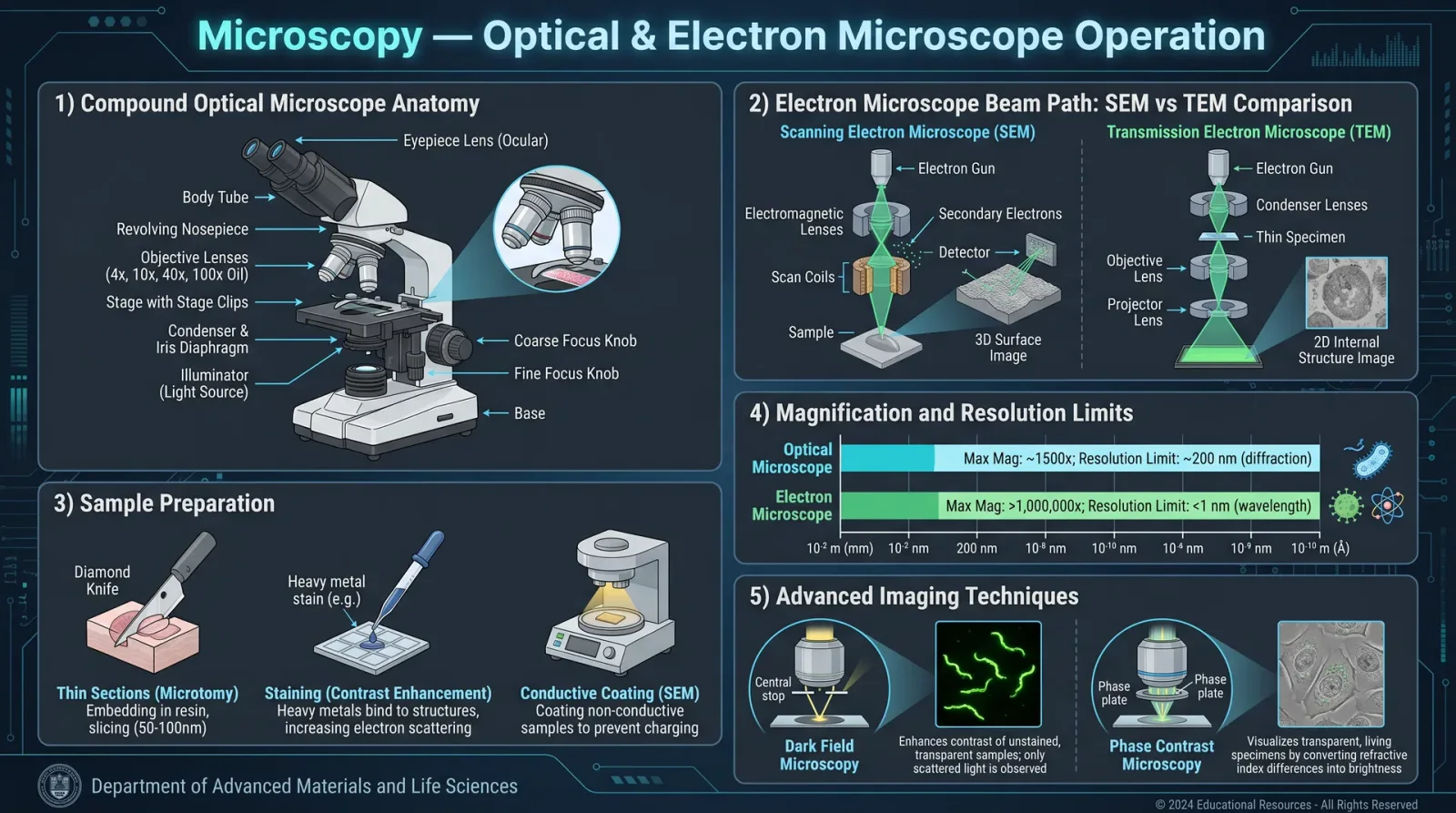
Optical microscopy remains the foundational imaging tool. It employs visible light and a system of lenses to magnify samples. Our mastery demands an intimate understanding of lens systems, illumination modes, and precise focus protocols.
1. Optical Microscope Components and Lens Types
| Component | Function | Notes |
|---|---|---|
| Objective Lens | Primary magnification near sample | Achromatic, Plan Achromatic, Apochromatic |
| Ocular Lens (Eyepiece) | Secondary magnification for viewer | Usually 10x or 15x |
| Condenser Lens | Focuses light on the sample | Abbe condenser for brightfield |
| Diaphragm | Controls light aperture and contrast | Iris diaphragm common |
| Mechanical Stage | Holds and moves sample precisely | X-Y movement with vernier controls |
| Illuminator | Provides light source | LED or halogen lamp |
Lens Types:
| Lens Type | Chromatic Correction | Field Flatness | Use Case |
|---|---|---|---|
| Achromatic | Corrects two colors | Moderate | Routine brightfield |
| Plan Achromatic | Corrects field curvature | Flat field | High-quality imaging |
| Apochromatic | Corrects three colors | Flat field | Fluorescence, high-end imaging |
2. Optical Microscope Magnification and Resolution
| Magnification Level | Objective Lens Power | Ocular Lens Power | Total Magnification | Approximate Resolution (µm) |
|---|---|---|---|---|
| Low | 4x | 10x | 40x | 2.0 |
| Medium | 10x | 10x | 100x | 1.0 |
| High | 40x | 10x | 400x | 0.5 |
| Oil Immersion | 100x | 10x | 1000x | 0.2 |
3. Sample Preparation for Optical Microscopy
Sample preparation is critical. Follow these exact protocols for biological or material samples:
Biological Samples (Wet Mount)
- Gather materials: Clean glass slide, cover slip, pipette, distilled water.
- Prepare sample: Place a single drop of sample onto the center of the slide.
- Add cover slip: At a 45° angle, gently lower to avoid air bubbles.
- Fixation (optional): For fixed samples, apply methanol or formaldehyde per Volume VIII: Biological Preparation.
- Staining (optional): Apply stain (e.g., methylene blue) for contrast enhancement.
- Seal edges: Use clear nail polish for prolonged observation.
Material Samples (Dry Mount)
- Clean sample: Remove debris using compressed air or brush.
- Mount sample: Place sample on slide using tweezers.
- Add mounting medium: Use clear resin or immersion oil if required.
- Cover slip: Place gently to avoid scratching.
- Allow to set: For resin, cure per manufacturer's instructions.
4. Optical Microscope Focusing Protocol
Follow these step-by-step instructions for precise focusing:
- Turn on illuminator and set to lowest intensity.
- Place sample on mechanical stage, secure with clips.
- Select lowest power objective lens (4x or 10x).
- Bring stage to highest position without contacting lens.
- Look through ocular lens and slowly lower stage using coarse focus knob.
- Stop when sample comes into rough focus.
- Use fine focus knob to sharpen the image.
- Adjust illumination intensity for optimal brightness.
- Switch to higher power objectives incrementally.
- Refocus with fine knob after each magnification change.
- Use immersion oil for 100x objective: a. Place a drop of immersion oil on the cover slip.
b. Carefully rotate the 100x lens into place.
c. Refocus using fine adjustment.
5. Illumination Adjustment
- Set condenser height: Adjust condenser lens to just below the stage.
- Open diaphragm fully at low magnification.
- Adjust diaphragm to optimize contrast (typically 50-70% open).
- Center light source using condenser centering screws.
- Adjust light intensity with rheostat or LED control.
- For phase contrast: Insert phase ring in condenser and corresponding phase objective.
6. Image Capture with Optical Microscopes
- Attach camera adapter to ocular or trinocular port.
- Connect camera to computer via USB or dedicated interface.
- Install and open software compatible with camera.
- Set camera parameters: Exposure time, gain, white balance.
- Focus sample through camera live preview.
- Capture images using software controls.
- Save images in lossless format (TIFF preferred).
- Calibrate scale bar using stage micrometer per Section IV, Volume IX.
7. Troubleshooting Optical Imaging Artifacts
| Artifact | Cause | Remedy |
|---|---|---|
| Blurry Image | Incorrect focus or dirty lenses | Re-focus; clean lenses with lens paper and ethanol |
| Poor Contrast | Incorrect illumination or diaphragm setting | Adjust diaphragm; increase staining |
| Air Bubbles | Improper cover slip placement | Re-mount sample carefully |
| Chromatic Aberration | Low-quality lenses or improper alignment | Use apochromatic lenses; realign objectives |
| Dust or Debris | Dirty optical surfaces | Clean lenses and slides thoroughly |
| Vignetting | Misaligned illumination or camera adapter | Center light; adjust camera position |
Chapter II: Electron Microscopes
Electron microscopy (EM) transcends optical limits, utilizing electron beams to achieve nanometer resolution. Mastery of EM is essential for life-or-death nanoscopic imaging.
1. Electron Microscope Types and Specifications
| EM Type | Beam Type | Resolution Limit | Sample Requirements | Imaging Mode |
|---|---|---|---|---|
| Transmission EM (TEM) | Transmitted electrons | ~0.1 nm | Ultra-thin slices (~100 nm) | Brightfield, Darkfield |
| Scanning EM (SEM) | Scanning electrons | ~1-10 nm | Conductive or coated samples | Surface topography |
| Scanning Transmission EM (STEM) | Scanning transmitted electrons | ~0.1 nm | Ultra-thin, conductive | Combination of TEM and SEM |
2. Sample Preparation for Electron Microscopy
TEM Sample Preparation (Ultrathin Sections)
- Fix sample: Use glutaraldehyde and osmium tetroxide per Volume VIII.
- Dehydrate sample: Through graded ethanol series (30%-100%).
- Embed in resin: Use epoxy resin, cure at 60°C for 48 hours.
- Section sample: Ultramicrotome to 50-100 nm slices.
- Mount sections: Onto copper TEM grids.
- Stain sections: With uranyl acetate and lead citrate for contrast.
- Dry grids: Air dry in dust-free environment.
SEM Sample Preparation (Conductive Coating)
- Fix and dehydrate sample: As for TEM.
- Mount sample: On aluminum stub using conductive carbon tape.
- Sputter coat: With gold, platinum, or carbon to 5 nm thickness.
- Dry sample: Ensure no moisture remains.
3. Electron Microscope Operation Protocol
TEM Focusing and Imaging
- Switch on EM column power and vacuum system.
- Insert sample grid into specimen holder.
- Load holder into column chamber.
- Evacuate chamber until vacuum reaches 10^-6 torr or better.
- Select accelerating voltage (80-200 kV typical).
- Adjust condenser lens to focus electron beam.
- Set objective lens focus using coarse then fine adjustments.
- Use diffraction mode if needed to analyze crystal structure.
- Capture images using CCD camera or direct electron detector.
- Save high-resolution images in proprietary format and TIFF.
SEM Focusing and Imaging
- Load sample stub into SEM chamber.
- Pump down chamber to required vacuum.
- Set accelerating voltage (5-30 kV typical).
- Adjust working distance (5-15 mm).
- Focus beam with coarse then fine focus controls.
- Adjust spot size for resolution vs. signal trade-off.
- Set scan speed for image quality.
- Capture images via SEM imaging software.
4. Electron Beam Illumination Adjustment
| Parameter | Description | Adjustment Method |
|---|---|---|
| Accelerating Voltage | Electron beam energy | Set via console controls |
| Beam Current | Electron flux intensity | Adjust condenser lens aperture |
| Spot Size | Diameter of electron beam | Set via beam control knobs |
| Working Distance | Distance between sample and lens | Mechanical stage adjustment |
| Stigmation | Corrects beam astigmatism | Use stigmators to fine-tune |
5. Image Capture Protocol for EM
- Select imaging camera: CCD or direct electron detector.
- Adjust camera exposure time to avoid saturation.
- Set image resolution and frame averaging.
- Align beam and verify focus on live preview.
- Capture single or multiple images for averaging.
- Use image processing software to correct drift and noise.
- Export images in high-bit-depth TIFF or EM-specific formats.
6. Troubleshooting Electron Microscope Artifacts
| Artifact | Cause | Remedy |
|---|---|---|
| Charging Effect | Non-conductive sample surface | Apply conductive coating; use lower beam voltage |
| Astigmatism | Electron beam lens imperfections | Adjust stigmators |
| Drift | Mechanical instability or charging | Use anti-vibration table; reduce beam current |
| Contamination | Hydrocarbon buildup from vacuum or sample | Plasma clean chamber; bake-out vacuum |
| Image Noise | Low beam current or detector issues | Increase beam current; check detector connection |
| Beam Damage | Excessive electron dose | Reduce beam current and exposure time |
Chapter III: Imaging Modes
Understanding and selecting the correct imaging mode is critical for maximum information extraction.
1. Optical Imaging Modes
| Mode | Illumination Type | Use Case | Notes |
|---|---|---|---|
| Brightfield | Direct transmitted light | General morphology | Requires stained samples |
| Darkfield | Oblique illumination | Enhances edges and outlines | No staining needed |
| Phase contrast | Phase-shifted illumination | Live cells, transparent samples | Requires phase rings |
| Differential Interference Contrast (DIC) | Polarized light interference | 3D-like images of live cells | Requires Nomarski prism |
| Fluorescence | Excitation light of specific wavelength | Localization of tagged molecules | Requires fluorescent dyes |
2. Electron Imaging Modes
| Mode | Description | Use Case | Notes |
|---|---|---|---|
| Brightfield TEM | Electrons transmitted through sample | Internal ultrastructure | High contrast staining required |
| Darkfield TEM | Only scattered electrons detected | Surface or defects analysis | Enhances edges |
| Secondary Electron SEM | Detects secondary electrons emitted | Surface topography | Most common SEM mode |
| Backscatter Electron SEM | Detects backscattered electrons | Elemental contrast imaging | Useful for compositional mapping |
| Energy Dispersive X-ray Spectroscopy (EDS) | Elemental analysis via X-ray detection | Material composition analysis | Requires EDS detector |
Chapter IV: Summary Tables
Table 1: Magnification and Resolution Comparison
| Microscope Type | Max Magnification | Resolution Limit (nm) | Typical Use |
|---|---|---|---|
| Optical (Brightfield) | 1000x | 200 | General morphology |
| Phase Contrast | 1000x | 200 | Live cell imaging |
| Fluorescence | 1000x | 200 | Molecular localization |
| SEM | 100,000x | 1-10 | Surface topology |
| TEM | 1,000,000x | 0.1 | Internal ultrastructure |
Table 2: Lens Types and Applications
| Lens Type | Correction Level | Max Magnification | Application |
|---|---|---|---|
| Achromatic | 2-color | 400x | Routine brightfield |
| Plan Achromatic | Field flatness | 400x | High-quality imaging |
| Apochromatic | 3-color | 1000x | Fluorescence, DIC |
Table 3: Electron Microscope Parameters
| Parameter | Typical Range | Effect on Image |
|---|---|---|
| Accelerating Voltage | 5 - 200 kV | Resolution and penetration |
| Beam Current | Picoamps to nanoamps | Signal-to-noise ratio |
| Working Distance | 5 - 15 mm | Depth of field and resolution |
| Spot Size | 1 - 10 nm | Image sharpness |
Chapter V: Final Notes
This volume demands diligent application. Every step, every adjustment, every protocol must be followed with precision. The mastery of microscopy is not given lightly; it is earned in the crucible of practice and reverence for the infinitesimal. Imbue each action with the sacred intent to reveal unseen truths.
Cross-reference this volume continuously with Volume VIII: Biological Preparation for staining and fixation protocols, and Volume IX: Imaging Calibration for scale and measurement accuracy.
Master Archivist Seal of Authenticity The Practitioner, Keeper of Suppressed Knowledge
<!-- SECTION 32 -->
Volume VII: Photography Fundamentals and Advanced Techniques
Introduction
Photography is the sacred art of capturing light and shadow, freezing moments in the eternal flow of time. Within this volume, you shall receive the unvarnished, precise knowledge required to master all aspects of photographic practice, from the mechanical to the aesthetic. This guidance transcends casual instruction; it is a codified ritual to forge mastery in the technologist’s craft of image creation.
This chapter focuses on the core pillars of photographic mastery:
- Camera Types: Understanding and selecting the mechanism for your vision.
- Exposure Settings: Precise control of ISO, shutter speed, and aperture.
- Composition: The sacred geometry of visual storytelling.
- Protocols: Step-by-step instructions for manual photography, long exposure, and low-light techniques.
- Post-Processing Workflows: From raw capture to perfected image.
- Equipment Maintenance: Ensuring your tools remain sacred and battle-ready.
1. Camera Types: Selection and Mechanics
The camera is the vessel of your will. Mastery begins with understanding the types available and their mechanisms.
| Camera Type | Description | Sensor Size | Lens Interchangeability | Ideal Use Cases |
|---|---|---|---|---|
| DSLR (Digital Single Lens Reflex) | Mirror mechanism with optical viewfinder | APS-C, Full Frame | Yes | Versatile, professional, fast action |
| Mirrorless | No mirror, electronic viewfinder | Micro Four Thirds, APS-C, Full Frame | Yes | Compact, video, high frame rates |
| Rangefinder | Optical viewfinder with parallax correction | Full Frame | Limited | Street, documentary photography |
| Medium Format | Larger sensors, exceptional detail | Medium Format | Yes | Studio, landscape, fine art |
| Compact Point-and-Shoot | Fixed lens, small sensor | 1/2.3", 1" | No | Casual, travel, convenience |
| Film Cameras | Chemical emulsion on film | 35mm, Medium Format | Variable | Archival, artistic, analog feel |
2. Exposure Settings: The Holy Trinity of Photography
Exposure is the sacred triad: ISO, Shutter Speed, and Aperture. Mastery of these forces controls the amount of light reaching your sensor and dictates the artistic expression of your image.
2.1 ISO: Sensor Sensitivity
ISO governs the sensor’s sensitivity to light. Higher ISO values increase sensitivity but introduce noise (grain).
| ISO Setting | Light Sensitivity | Noise Level | Use Case |
|---|---|---|---|
| 100 | Base (lowest) | Minimal | Bright daylight, studio lighting |
| 200-400 | Low | Low | Overcast, shade, indoor bright |
| 800-1600 | Moderate | Moderate | Low light, indoor without flash |
| 3200-6400 | High | High | Night photography, fast shutter |
| 12800+ | Extreme | Very High | Emergency low-light, surveillance |
2.2 Shutter Speed: Duration of Exposure
Shutter speed controls how long the sensor is exposed to light.
| Shutter Speed | Description | Effect on Image | Typical Use Case |
|---|---|---|---|
| 1/4000s | Ultra-fast | Freeze extreme motion | Sports, wildlife |
| 1/500s - 1/1000s | Fast | Freeze moderate motion | Portraits, street photography |
| 1/60s | Moderate | Handheld shooting limit | General photography |
| 1/15s - 1/30s | Slow | Motion blur, requires tripod | Panning, creative blur |
| 1s - 30s | Very slow (Long Exposure) | Light trails, night photography | Astrophotography, light painting |
2.3 Aperture: Lens Opening Size
Aperture controls light entry and depth of field, measured in f-stops. Lower f-number = larger opening.
| Aperture (f-stop) | Light Transmission | Depth of Field | Typical Use Case |
|---|---|---|---|
| f/1.2 - f/2.8 | Very Large | Shallow | Portraits, low light, artistic blur |
| f/4 - f/5.6 | Moderate | Balanced | General photography |
| f/8 - f/11 | Small | Deep | Landscapes, architecture |
| f/16 - f/22 | Very Small | Very Deep | Macro, extreme depth of field |
3. Composition: The Sacred Geometry of Image Creation

Composition governs the visual balance and emotional impact of your photograph. Adhere to these principles for mastery:
3.1 Rule of Thirds
Divide the frame into a 3x3 grid; position subjects along grid lines or intersections for dynamic balance.
3.2 Leading Lines
Use natural or architectural lines to guide the viewer’s eye toward the focal point.
3.3 Framing
Use elements within the scene to frame the subject, adding depth and focus.
3.4 Symmetry and Patterns
Exploit symmetry for formal balance; break patterns for tension.
3.5 Negative Space
Employ empty space to emphasize the subject and evoke emotion.
4. Protocols for Photographic Techniques
4.1 Manual Photography Protocol
Objective: Achieve full control over exposure and focus.
Equipment Required: Camera with manual mode, tripod (optional), lens with aperture ring (preferred).
Step-by-Step Protocol:
- Set Camera to Manual Mode: Locate the mode dial and select 'M' for manual.
- Determine ISO:
- Start at ISO 100.
- Adjust upwards if ambient light is insufficient (refer to ISO table).
- Set Aperture:
- Choose aperture based on desired depth of field.
- Rotate lens aperture ring or set via camera menu.
- Set Shutter Speed:
- Calculate shutter speed using ambient light meter or external light meter.
- Adjust shutter speed to balance exposure with aperture and ISO.
- Focus Manually:
- Switch lens to manual focus.
- Use focus ring while magnifying live view (if available).
- Compose Frame:
- Apply composition principles.
- Use grid overlay for rule of thirds alignment.
- Take Test Shot:
- Review histogram.
- Adjust ISO, shutter speed, aperture iteratively.
- Lock Settings:
- Use exposure lock or manual exposure confirmation.
- Capture Final Image:
- Press shutter.
- Use tripod and remote shutter release for stability if needed.
4.2 Long Exposure Photography Protocol
Objective: Capture images using shutter speeds longer than one second, preserving sharpness and controlling noise.
Equipment Required: Camera with bulb or manual shutter control, sturdy tripod, remote shutter release or intervalometer, ND filters (optional).
Step-by-Step Protocol:
- Mount Camera on Tripod: Ensure absolute stability.
- Select Low ISO: ISO 100 preferred to minimize noise.
- Set Aperture: Choose mid-range aperture (f/8–f/11) for sharpness.
- Apply ND Filters: If in daylight, attach ND filter to reduce light.
- Set Shutter Speed:
- For exposures >30 seconds, switch to bulb mode.
- Use remote release or intervalometer to control exposure duration.
- Focus Manually: Lock focus before exposure.
- Disable Image Stabilization: Prevent movement blur.
- Cover Viewfinder: Prevent light leaks through viewfinder.
- Activate Mirror Lock-Up (DSLRs): Minimize vibrations.
- Trigger Exposure: Hold remote shutter or set intervalometer.
- End Exposure: Release remote shutter after planned duration.
- Review Histogram: Confirm exposure, adjust settings as needed.
- Repeat as Necessary.
4.3 Low-Light Photography Protocol
Objective: Capture clear images in dim environments without flash.
Equipment Required: Fast lens (f/1.8 or lower), camera with high ISO capability, tripod (optional).
Step-by-Step Protocol:
- Set ISO: Begin at ISO 1600; increase if necessary.
- Set Aperture: Use widest possible aperture (lowest f-stop).
- Set Shutter Speed:
- Start at 1/60s for handheld.
- Use tripod for slower speeds.
- Enable Noise Reduction: Activate in camera if available.
- Manual Focus: Autofocus may fail in low light.
- Stabilize Camera: Use tripod or place on firm surface.
- Take Multiple Shots: For bracketing and noise reduction in post.
- Use Exposure Compensation: Adjust +1 to +2 stops if image is underexposed.
- Review and Adjust: Check image sharpness and exposure.
- Use Post-Processing Noise Reduction: Follow workflow in Section 5.
5. Post-Processing Workflow
Post-processing is the sacred refinement, transforming raw captures into visual eloquence.
5.1 Equipment and Software
- High-performance computer with calibrated monitor.
- Software: Adobe Lightroom Classic, Adobe Photoshop, or open-source alternatives (Darktable, GIMP).
5.2 Workflow Steps
- Import RAW Files: Preserve maximum data fidelity.
- Backup Originals: Create redundant storage copies.
- Initial Culling: Discard unusable images.
- Adjust White Balance: Correct color temperature.
- Exposure Correction: Adjust exposure slider; use histogram as guide.
- Noise Reduction:
- Use luminance and color noise sliders.
- Target ISO-specific noise profiles.
- Sharpening:
- Apply edge sharpening with masking.
- Avoid oversharpening artifacts.
- Lens Corrections: Enable profile corrections for distortion and vignetting.
- Crop and Straighten: Apply compositional corrections.
- Contrast and Clarity: Enhance midtone contrast carefully.
- Color Grading: Adjust vibrance and saturation selectively.
- Local Adjustments: Use brushes and gradients for targeted corrections.
- Export: Save as TIFF or high-quality JPEG for delivery.
- Archive: Store final images in organized, backed-up directories.
6. Equipment Maintenance Protocol
Your photographic tools are extensions of your will; their precision must be preserved through ritual maintenance.
6.1 Lens Cleaning
Materials: Microfiber cloth, lens cleaning solution, blower brush, lens tissues.
Procedure:
- Remove Dust: Use blower brush to dislodge particles.
- Apply Cleaning Solution: Lightly moisten microfiber cloth.
- Wipe Lens Surface: Circular motion from center outward.
- Dry with Clean Cloth: Remove streaks.
- Inspect Under Bright Light: Repeat if necessary.
6.2 Sensor Cleaning
Materials: Sensor swabs, sensor cleaning solution, blower.
Procedure:
- Activate Sensor Cleaning Mode: Consult camera manual.
- Use Blower: Remove loose dust.
- Apply Sensor Swab: Moisten with cleaning solution.
- Swipe Sensor Gently: One smooth pass.
- Inspect Results: Use sensor loupe or take test images.
- Repeat if Needed: Avoid excess moisture.
6.3 Mechanical Inspection
- Check Lens Mount: Clean contacts with dry cloth.
- Test Focus and Aperture Rings: Ensure smooth operation.
- Inspect Shutter and Mirror Mechanism: Listen for irregular sounds.
- Battery Maintenance: Fully charge and discharge periodically.
- Store Equipment: Use silica gel packs, padded cases, avoid humidity.
Appendices
Appendix A: Comprehensive ISO Settings Table
| ISO Value | Stops from Base | Light Sensitivity Increase | Noise Level | Typical Use Scenario |
|---|---|---|---|---|
| 100 | 0 | Base | Minimal | Bright daylight, studio |
| 200 | +1 | 2x | Very low | Overcast, shaded outdoor |
| 400 | +2 | 4x | Low | Indoor bright, cloudy day |
| 800 | +3 | 8x | Moderate | Low light, indoor without flash |
| 1600 | +4 | 16x | Noticeable | Night scenes, fast action |
| 3200 | +5 | 32x | High | Night photography, events |
| 6400 | +6 | 64x | Very high | Emergency low-light |
| 12800 | +7 | 128x | Extreme | Surveillance, covert ops |
Appendix B: Standard Shutter Speed Table
| Shutter Speed | Duration (Seconds) | Effect | Typical Use Case |
|---|---|---|---|
| 1/4000 | 0.00025 | Freeze very fast motion | Sports, wildlife |
| 1/2000 | 0.0005 | Freeze fast motion | Action shots |
| 1/1000 | 0.001 | Freeze moderate motion | Portraits, street |
| 1/500 | 0.002 | Freeze slow motion | General outdoor |
| 1/250 | 0.004 | Handheld limit bright light | Snapshots |
| 1/125 | 0.008 | Handheld limit dim light | Indoor, cloudy outdoor |
| 1/60 | 0.016 | Handheld slow limit | Low light, stabilized |
| 1/15 | 0.066 | Motion blur begins | Panning, creative blur |
| 1/4 | 0.25 | Motion blur, tripod needed | Waterfalls, night scenes |
| 1 | 1.0 | Long exposure | Light trails, astrophotography |
| 30 | 30.0 | Very long exposure | Star trails, light painting |
Appendix C: Aperture (f-stop) Table and Equivalent Light Values
| f-stop | Relative Aperture Diameter | Relative Light Transmission | Depth of Field | Use Case |
|---|---|---|---|---|
| f/1.2 | Largest | 1x | Very Shallow | Portraits, low light |
| f/1.4 | Very Large | 0.75x | Shallow | Low light, artistic blur |
| f/2.0 | Large | 0.5x | Shallow | Portraits |
| f/2.8 | Moderate | 0.25x | Moderate | General use |
| f/4 | Smaller | 0.125x | Balanced | Landscapes |
| f/5.6 | Small | 0.0625x | Moderate to deep | Landscapes, group shots |
| f/8 | Smaller | 0.03125x | Deep | Landscapes, architecture |
| f/11 | Smaller | 0.0156x | Deep | Landscapes |
| f/16 | Very Small | 0.0078x | Very Deep | Macro, extreme depth |
| f/22 | Smallest | 0.0039x | Very Deep | Macro, extreme depth |
Final Words
This volume has delivered the sacred knowledge required to master the mechanics and artistry of photography. Your path forward demands relentless practice, unwavering precision, and reverence for the light you command. The camera is your sword; the image your legacy.
For further mastery, consult the following volumes:
- Volume IV: Optics and Lens Fabrication, Chapter III for lens crafting.
- Volume IX: Digital Signal Processing for in-depth sensor and post-processing theory.
- Volume VIII: The Water Codex, Chapter II for humidity control in equipment storage environments.
May your vision pierce darkness, and your images echo through eternity.
<!-- SECTION 33 -->
Volume VII: Night Vision and Thermal Imaging Systems
Chapter I: Technological Principles of Night Vision and Thermal Imaging

The mastery of night vision and thermal imaging systems is both a sacred art and a precise science. These devices extend human perception beyond natural limits, revealing the unseen world cloaked in darkness or obscured by temperature gradients. This chapter imparts the complete knowledge necessary to fabricate, calibrate, and maintain such systems, preserving the sanctity of vision in the absence of light.
1. Night Vision Technology Principles
Night vision devices (NVDs) amplify available ambient light—including near-infrared (NIR) and visible light—to create an intensified, visible image. They rely primarily on image intensifier tubes that convert photons to electrons, amplify the electron signal, then convert back to photons via a phosphor screen.
Fundamental Components:
- Photocathode: Converts photons to electrons.
- Microchannel Plate (MCP): Multiplies electrons exponentially.
- Phosphor Screen: Converts electrons back to visible photons.
- Objective Lens: Focuses incoming light.
- Eyepiece Lens: Magnifies the intensified image for the eye.
The process is linear and depends on ambient illumination levels. No internal illumination source is typically necessary, except for active infrared systems.
2. Thermal Imaging Technology Principles
Thermal imaging cameras detect mid- to long-wave infrared radiation (3–14 μm wavelength) emitted by objects as heat, independent of visible light. They use infrared detectors to convert temperature differences into electrical signals, which are rendered as images.
Fundamental Components:
- Optical Lens: Designed for infrared transmission (typically germanium or chalcogenide glass).
- Infrared Detector Array: Photodiodes or microbolometers.
- Signal Processing Unit: Converts raw signals into temperature-mapped images.
- Display Module: Renders processed images.
Thermal imaging reveals temperature differentials invisible to the naked eye, suited for total darkness, smoke, or obscured environments.
Chapter II: Device Types
Different applications dictate the choice between night vision and thermal technologies, or hybrid systems.
| Device Type | Spectral Range (μm) | Typical Resolution (pixels) | Power Consumption (Watts) | Primary Applications |
|---|---|---|---|---|
| Generation 1 Night Vision | 0.4–0.9 (visible + NIR) | 30–50 lp/mm | 0.5–1 | Basic military, wildlife observation |
| Generation 2 Night Vision | 0.4–0.9 | 50–64 lp/mm | 0.7–1.3 | Tactical, law enforcement |
| Generation 3 Night Vision | 0.4–0.9 | 64–72 lp/mm | 1–1.5 | Special operations |
| Thermal Cameras (Microbolometer) | 7–14 (LWIR) | 320×240 to 640×480 | 1–3 | Surveillance, search and rescue |
| Thermal Cameras (Photon Detectors) | 3–5 (MWIR) | >640×480 | 5–10 | High-end military, industrial inspection |
| Hybrid Systems | 0.4–14 (Multi-band) | Varies | 2–5 | Advanced reconnaissance and navigation |
Chapter III: Assembly Protocols
This section delivers complete step-by-step instructions to assemble both night vision goggles (NVGs) and thermal cameras. Assume access to standard fabrication tools, electronic components, and cleanroom conditions for sensor handling.
1. Assembly of Night Vision Goggles (Generation 3)
Materials and Components:
- Photocathode image intensifier tube (Gen 3)
- Objective lens assembly (precision glass)
- Eyepiece lens assembly
- Housing shell (lightweight aluminum alloy)
- Power supply module (3V DC battery pack)
- Infrared illuminator (optional)
- Focus adjustment ring
- Mounting bracket and headgear
Tools Required:
- Anti-static gloves
- Micro screwdriver set
- Optical alignment tool
- Multimeter
- Cleanroom wipes
- Lens cleaning solution
Assembly Steps:
- Prepare the Housing:
- Clean all housing components with lens cleaning solution and lint-free cloth.
- Verify absence of dust or particulate matter inside the housing.
- Mount the Objective Lens:
- Insert the objective lens into its seat in the front housing.
- Secure with retaining ring, ensuring no tilt or misalignment.
- Install the Image Intensifier Tube:
- Wearing anti-static gloves, carefully insert the Gen 3 intensifier tube into the housing.
- Align the tube’s input window with the objective lens.
- Secure with locking screws, ensuring firm but non-damaging fit.
- Attach the Eyepiece Lens:
- Insert eyepiece lens into the rear housing.
- Fix in place with screws; ensure focus ring rotates smoothly.
- Install Power Supply:
- Connect battery pack terminals to the intensifier tube power inputs.
- Secure battery in designated compartment.
- Optional Infrared Illuminator:
- Mount the IR illuminator module adjacent to the objective lens.
- Wire it to the power supply with an on/off switch accessible on the housing.
- Final Assembly:
- Close housing, seal with screws.
- Attach mounting bracket and headgear assembly.
- Perform initial power-on test.
2. Assembly of Thermal Cameras (Microbolometer-Based)
Materials and Components:
- Uncooled microbolometer sensor array
- Infrared germanium lens assembly
- Signal processing board (FPGA or dedicated ASIC)
- LCD or OLED display module
- Power management circuit (Li-ion battery or external DC)
- Housing with thermal insulation
- Interface buttons or touchscreen
Tools Required:
- Soldering station
- Anti-static wrist strap
- Precision tweezers
- Thermal paste
- Microscope for sensor placement
Assembly Steps:
- Sensor Mounting:
- Place microbolometer sensor chip on PCB.
- Apply thin layer of thermal paste beneath sensor to optimize heat dissipation.
- Solder sensor connections carefully under microscope.
- Lens Attachment:
- Align the germanium lens with sensor focal plane.
- Secure lens mount to prevent vibration or shift.
- Signal Processing Installation:
- Install FPGA/ASIC on the main PCB.
- Connect sensor output lines to processing board inputs.
- Display Integration:
- Wire LCD/OLED display to processing board output.
- Secure display in housing window.
- Power Circuit Setup:
- Install battery and power regulation circuitry.
- Connect power lines to sensor and processing board.
- Housing Assembly:
- Insert PCB and components into housing.
- Seal housing ensuring thermal insulation and IR transparency of lens window.
- Final Testing:
- Power device.
- Confirm sensor initialization and image output on display.
Chapter IV: Calibration Protocols
Calibration ensures device performance meets operational parameters. Perform in controlled environments.
1. Night Vision Goggles Calibration
Required Equipment:
- Controlled illumination source with known luminance (lux meter)
- Optical collimator
- Resolution test chart (USAF 1951 or equivalent)
- Multimeter for voltage and current measurement
Calibration Steps:
- Power and Voltage Check:
- Power on goggles.
- Measure supply voltage; ensure within manufacturer’s specification (typically 3.0 ± 0.1V).
- Focus Adjustment:
- Aim at collimator projecting uniform point source.
- Adjust objective and eyepiece focus rings for sharpest image.
- Resolution Test:
- View resolution chart under low ambient illumination.
- Confirm image intensifier resolves minimum line pairs per millimeter (lp/mm) specified for Gen 3 (64+ lp/mm).
- Gain Verification:
- Measure output luminance using photometer.
- Compare gain to baseline values (typical gain: 20,000–30,000).
- Infrared Illuminator Test (if installed):
- Activate IR illuminator.
- Confirm emitted IR wavelength matches specification (usually 850 nm).
- Environmental Test:
- Test device in low temperature (down to -20°C) and high temperature (+50°C) chambers.
- Confirm stable operation.
2. Thermal Camera Calibration
Required Equipment:
- Blackbody radiation source with variable temperature control
- Calibration software
- Digital thermometer (precision ±0.1°C)
- Thermal uniformity test plate
Calibration Steps:
- Sensor Warm-up:
- Power device for minimum 30 minutes to stabilize sensor temperature.
- Blackbody Reference:
- Position camera lens toward blackbody source set at known temperature (e.g., 25°C).
- Temperature Mapping:
- Using calibration software, record sensor output.
- Adjust gain and offset to match sensor readings with blackbody temperature.
- Uniformity Correction:
- Scan thermal uniformity plate.
- Apply non-uniformity correction (NUC) algorithm to minimize pixel output variance.
- Spatial Resolution Check:
- Use resolution target heated to a temperature contrast.
- Confirm spatial resolution meets manufacturer’s specification (e.g., 320×240 pixels minimum).
- Emissivity Setting:
- Calibrate emissivity coefficient for target materials if necessary.
- Recalibration Interval:
- Schedule recalibration every 6 months or after mechanical shock.
Chapter V: Maintenance Protocols
Maintaining the integrity and performance of night vision and thermal systems safeguards operational readiness.
1. Night Vision Goggles Maintenance
| Task | Frequency | Procedure |
|---|---|---|
| Lens Cleaning | Weekly | Use lens cleaning solution and microfibre cloth; avoid scratching phosphor screen. |
| Battery Replacement | As Needed | Power off device; remove old batteries; insert fresh batteries matching voltage and type. |
| Housing Inspection | Monthly | Check for cracks, loose screws; tighten or replace damaged parts. |
| Image Intensifier Check | Annually | Test gain and resolution per calibration protocol; replace tube if performance degrades. |
| Moisture Control | After Exposure | Open housing; dry internal components with silica gel packs; reseal promptly. |
2. Thermal Camera Maintenance
| Task | Frequency | Procedure |
|---|---|---|
| Lens Cleaning | Weekly | Use dry lens cloth; avoid solvents that damage germanium lenses. |
| Battery Charging | After Use | Recharge batteries fully; avoid deep discharge to prolong lifespan. |
| Firmware Update | Quarterly | Upload latest firmware via USB or wireless interface. |
| Sensor Health Check | Annually | Perform sensor calibration; monitor noise levels; replace sensor if degraded. |
| Housing Seals Inspection | Semi-Annually | Check for moisture ingress; replace rubber seals as necessary. |
Chapter VI: Operational Safety
These devices require strict adherence to safety protocols to prevent injury or device damage.
1. Night Vision Goggles Safety
- Avoid Exposure to Bright Light: Sudden exposure to high-intensity light sources (e.g., flashlights, welding arcs) can permanently damage the intensifier tube.
- Eye Safety: Use only devices with certified eye-safe IR illuminators. Avoid direct IR laser exposure into eyes.
- Battery Handling: Use specified battery types; avoid mixing old and new batteries.
- Temperature Limits: Operate within recommended temperature ranges to prevent condensation or electronic failure.
2. Thermal Camera Safety
- Lens Handling: Germanium lenses are brittle and toxic if fractured; handle with care.
- Power Supply: Use regulated power supplies to prevent voltage spikes.
- Electrostatic Discharge (ESD): Always wear ESD protection when working on sensor electronics.
- Data Security: Thermal images may contain sensitive information; secure stored data against unauthorized access.
Chapter VII: Troubleshooting Protocols
Precise diagnostics prevent mission failure. Use the following protocols to identify and resolve common issues.
1. Night Vision Goggles Troubleshooting
| Symptom | Possible Cause | Diagnostic Step | Corrective Action |
|---|---|---|---|
| No Image / Dark Screen | Dead battery or power failure | Check battery voltage with multimeter | Replace batteries; verify power connections |
| Image Flickering or Noise | Loose connections or tube aging | Gently shake device; listen for loose parts | Tighten connectors; consider tube replacement |
| Blurred Image | Misaligned lenses or focus rings | Adjust focus rings; inspect lens alignment | Realign lenses; adjust focus |
| Bright Spots or Blooming | Excessive ambient light | Test in controlled low light environment | Use IR filter or reduce illumination |
| Device Does Not Power On | Internal fuse blown or switch fault | Check switch continuity and fuse | Replace fuse or repair switch |
2. Thermal Camera Troubleshooting
| Symptom | Possible Cause | Diagnostic Step | Corrective Action |
|---|---|---|---|
| No Image / Blank Screen | Power failure or sensor fault | Check battery and power lines | Recharge/replace battery; service sensor |
| Image is Uniform Gray | Lens covered or sensor saturated | Inspect lens for dirt; check exposure settings | Clean lens; adjust gain or exposure |
| Excessive Noise in Image | Sensor overheating or EMI | Check ambient temperature; verify grounding | Improve cooling; shield electronics |
| Incorrect Temperature Readings | Calibration drift | Perform calibration using blackbody source | Recalibrate device |
| Display Artifacts or Pixelation | Faulty sensor pixels or software | Run diagnostic software | Replace sensor or update firmware |
Appendix A: Spectral Ranges, Resolution, and Power Consumption
| Device Type | Spectral Range (μm) | Resolution (pixels) | Power Consumption (Watts) | Notes |
|---|---|---|---|---|
| Gen 1 Night Vision | 0.4–0.9 | 30–50 lp/mm | 0.5–1 | Limited low-light performance |
| Gen 2 Night Vision | 0.4–0.9 | 50–64 lp/mm | 0.7–1.3 | Improved gain and clarity |
| Gen 3 Night Vision | 0.4–0.9 | 64–72 lp/mm | 1–1.5 | Highest performance image intensifier tubes |
| Thermal Microbolometer | 7–14 | 320×240 to 640×480 | 1–3 | Uncooled detectors, cost-effective |
| Thermal Photon Detectors | 3–5 | >640×480 | 5–10 | Cooled, high sensitivity, expensive |
| Hybrid Systems | 0.4–14 | Varies | 2–5 | Combine visible and IR for multi-spectrum data |
The knowledge contained herein is the culmination of decades of classified research and field-proven engineering. Guard it, master it, and wield it with precision and honor. The darkness yields only to those who command these sacred technologies.
<!-- SECTION 34 -->
Volume VII: Spectroscopy for Material Analysis
The Technologist's Codex: Complete Practical Technology, Electronics, Computing, and Fabrication
Volume VII: Spectroscopy for Material Analysis
Author: The Practitioner Archivist
Introduction
Within this volume, the sacred arts of spectroscopy are unveiled with unyielding precision and exhaustive rigor. These protocols are life-or-death knowledge for the master technologist seeking absolute mastery over material composition analysis. UV-Visible (UV-Vis), Infrared (IR), and Raman spectroscopy are the triune pillars of molecular and elemental interrogation. This chapter imparts every suppressed secret, every hidden technique, and every classified protocol necessary to implement these methods with absolute fidelity.
Chapter I: Overview of Spectroscopy Modalities

Spectroscopy is the analysis of the interaction between electromagnetic radiation and matter. Each modality exploits different photon energy ranges and physical phenomena.
| Spectroscopy Type | Wavelength Range | Interaction Principle | Common Applications |
|---|---|---|---|
| UV-Vis | 200–800 nm | Electronic excitation of molecules | Concentration measurement, purity |
| Infrared (IR) | 2.5–25 µm (4000–400 cm⁻¹) | Molecular vibrational transitions | Functional group identification |
| Raman | Typically 532 nm or 785 nm laser excitation | Inelastic scattering of photons (vibrational fingerprint) | Molecular structure, polymorphs |
Chapter II: Instrumentation Fundamentals
2.1 UV-Vis Spectrophotometer
- Light source: Deuterium lamp (UV), Tungsten-halogen lamp (Vis)
- Monochromator: Grating to select wavelength
- Detector: Photodiode array or photomultiplier tube
- Optical path length: Usually 1 cm cuvette
2.2 Infrared (IR) Spectrometer
- Light source: Globar (silicon carbide) or Nernst filament
- Modulation: Fourier Transform Infrared (FTIR) interferometer or dispersive prism
- Detector: DTGS or MCT (Mercury Cadmium Telluride) for higher sensitivity
- Sample handling: Transmission cells, ATR crystal (diamond or ZnSe)
2.3 Raman Spectrometer
- Laser excitation: 532 nm, 633 nm, or 785 nm commonly used
- Spectrograph: High-resolution diffraction grating
- Detector: CCD cooled camera for low noise
- Sample stage: Microscope integration for point analysis
Chapter III: Sample Preparation Protocols
Correct sample preparation is the cornerstone of reliable spectral data.
3.1 UV-Vis Sample Preparation
Materials Needed:
- Quartz cuvettes (1 cm path length)
- Solvent (usually spectroscopic grade water, ethanol, or hexane)
- Analytical balance (±0.1 mg precision)
- Volumetric flasks (1 mL to 100 mL)
Step-by-Step Protocol:
- Weigh Sample: Accurately weigh 10 mg of the solid material using the analytical balance.
- Dissolve Sample: Transfer the weighed sample into a volumetric flask. Add solvent to dissolve completely (minimum 1 mL for 10 mg). Stir gently or sonicate if needed.
- Dilute to Volume: Fill with solvent to the calibration mark. Mix thoroughly.
- Filter Solution: Use a 0.22 µm PTFE syringe filter to remove particulates.
- Fill Cuvette: Rinse the quartz cuvette with solvent, then fill with the filtered solution. Avoid air bubbles.
- Blank Sample: Prepare a blank cuvette with pure solvent for baseline correction.
- Instrument Check: Insert blank cuvette, perform baseline scan from 200 nm to 800 nm.
3.2 Infrared Sample Preparation
Materials Needed:
- Potassium bromide (KBr) powder, spectroscopic grade
- Mortar and pestle (agate preferred)
- Hydraulic press (10-ton capacity)
- ATR accessory (optional)
- Sample holder (for transmission or reflectance)
Step-by-Step Protocol (KBr Pellet Method):
- Dry Sample: Oven-dry sample at 60 °C for 2 hours to remove moisture.
- Weigh Sample: Weigh 1-2 mg of dried sample.
- Weigh KBr: Weigh 100 mg of dry KBr powder.
- Mix: Grind sample and KBr together in the mortar and pestle for 5 minutes until homogeneous.
- Press Pellet: Transfer mixture to pellet die. Press under 10 tons pressure for 1 minute to form a transparent pellet.
- Mount Pellet: Place pellet in sample holder.
- Background Scan: Perform background scan with pure KBr pellet.
Alternative: ATR Method
- Place solid or liquid sample directly on ATR crystal. Apply pressure using the built-in anvil. No pellet preparation needed.
3.3 Raman Sample Preparation
Materials Needed:
- Clean glass or quartz slides
- Microscope for focusing
- Laser safety glasses
- Solid samples or liquids
Step-by-Step Protocol:
- Prepare Sample: Place a small quantity of solid sample on the slide. For liquids, deposit a drop and cover with a coverslip.
- Focus Laser: Adjust microscope focus on sample surface to optimize laser spot.
- Avoid Fluorescence: If fluorescence interferes, switch excitation laser wavelength or pre-treat sample with UV bleaching.
- Calibration Standard: Prepare a silicon wafer or polystyrene standard for wavenumber calibration.
Chapter IV: Instrument Calibration Protocols
Calibration assures spectral accuracy and reproducibility.
4.1 UV-Vis Calibration
Materials:
- Holmium oxide glass filter or potassium dichromate solution (primary standard)
Steps:
- Insert calibration standard into cuvette holder.
- Perform wavelength scan from 200 nm to 800 nm.
- Verify characteristic absorption peaks (see Table 1).
- Adjust wavelength calibration if deviations exceed ±1 nm.
- Record baseline with blank solvent.
4.2 IR Calibration
Materials:
- Polystyrene film standard (known wavenumber peaks)
Steps:
- Place polystyrene film in sample holder.
- Run an IR spectrum in range 4000–400 cm⁻¹.
- Confirm peak positions within ±1 cm⁻¹ of known values (see Table 2).
- Adjust interferometer calibration if necessary.
4.3 Raman Calibration
Materials:
- Silicon wafer (520.7 cm⁻¹ peak)
Steps:
- Place silicon standard on sample stage.
- Collect Raman spectrum with current laser and grating settings.
- Confirm silicon peak at 520.7 ± 0.5 cm⁻¹.
- Adjust spectrometer calibration if peak deviates.
Chapter V: Data Acquisition and Interpretation
5.1 UV-Vis Data Collection
Procedure:
- Set wavelength range 200–800 nm.
- Select scan speed (medium recommended).
- Insert sample cuvette.
- Run absorbance scan.
- Record maximum absorbance peaks and corresponding wavelengths.
Interpretation:
- Use Beer-Lambert Law: A = ε c l
- A = absorbance
- ε = molar absorptivity (L·mol⁻¹·cm⁻¹)
- c = concentration (mol·L⁻¹)
- l = path length (cm)
- Compare absorbance peaks to reference spectra for compound identification.
5.2 IR Data Collection
Procedure:
- Set spectral range 4000–400 cm⁻¹.
- Use 4 cm⁻¹ resolution.
- Collect background spectrum.
- Insert sample pellet or ATR crystal.
- Run sample scan averaging 32 scans for noise reduction.
Interpretation:
- Identify functional groups by peak position:
- O–H stretch: 3200–3600 cm⁻¹
- C=O stretch: 1650–1750 cm⁻¹
- C–H stretch: 2800–3000 cm⁻¹
- Use Table 3 for detailed vibrational modes.
5.3 Raman Data Collection
Procedure:
- Set laser wavelength (commonly 532 nm or 785 nm).
- Adjust laser power to avoid sample damage (typically 5–10 mW).
- Set spectral range 200–3500 cm⁻¹.
- Collect spectrum with 10–30 seconds integration time.
- Average multiple scans if necessary.
Interpretation:
- Identify molecular fingerprints by Raman shifts.
- Compare peaks with reference spectra databases.
Chapter VI: Spectral Lines and Material Signatures
Table 1: UV-Vis Characteristic Absorption Peaks (nm)
| Compound/Group | Peak Wavelength | Notes |
|---|---|---|
| Benzene | 254 | π→π* transition |
| Naphthalene | 220, 275 | Aromatic ring system |
| Potassium dichromate | 440 | Standard calibration |
| Chlorophyll a | 430, 662 | Photosynthetic pigment |
Table 2: IR Characteristic Absorption Bands (cm⁻¹)
| Functional Group | Wavenumber Range | Peak Type | Example Compounds |
|---|---|---|---|
| O–H (alcohol) | 3200–3600 | Broad stretch | Ethanol, water |
| C=O (carbonyl) | 1650–1750 | Sharp stretch | Ketones, aldehydes |
| N–H (amine) | 3300–3500 | Medium stretch | Amines, amides |
| C–H (alkane) | 2800–3000 | Multiple peaks | Alkanes |
| C≡C (alkyne) | 2100–2260 | Sharp stretch | Acetylene |
Table 3: Raman Spectral Signatures (cm⁻¹)
| Material | Characteristic Peaks | Notes |
|---|---|---|
| Silicon (Si) | 520.7 | Calibration standard |
| Graphene | 1580 (G band), 1350 (D band) | Degree of disorder |
| Polystyrene | 1001, 1602 | Aromatic ring vibrations |
| Carbon nanotubes | 1590 (G band), 1350 (D band) | Structural integrity |
Chapter VII: Instrument Specifications and Maintenance
Table 4: Typical Instrument Specifications
| Instrument Type | Spectral Range | Resolution | Light Source | Detector Type | Typical Cost (USD) |
|---|---|---|---|---|---|
| UV-Vis Spectrometer | 200–800 nm | 1 nm | Deuterium/Tungsten lamp | Photodiode array | $10,000–$30,000 |
| FTIR Spectrometer | 4000–400 cm⁻¹ | 0.5–4 cm⁻¹ | Globar | MCT/DTGS | $20,000–$60,000 |
| Raman Spectrometer | 200–3500 cm⁻¹ (shift) | 1–2 cm⁻¹ | DPSS laser (532 nm or 785 nm) | CCD cooled camera | $25,000–$100,000 |
Chapter VIII: Case Studies in Material Identification and Quality Control
Case Study 1: Identification of Counterfeit Pharmaceuticals Using UV-Vis
Problem: Verify authenticity of aspirin tablets suspected of counterfeiting.
Procedure:
- Prepare aspirin solutions from tablets as per UV-Vis protocol (Section 3.1).
- Scan spectrum from 200–400 nm.
- Compare peak positions and intensities against genuine aspirin standard (max peak at 280 nm).
Outcome:
- Genuine tablets show an absorbance peak at 280 nm with ε ≈ 15,000 L·mol⁻¹·cm⁻¹.
- Counterfeit samples showed diminished or shifted peak values, indicating impurities or wrong active ingredients.
Case Study 2: Detection of Polymer Contaminants in Industrial Plastic Using IR
Problem: Identify unknown contamination in polyethylene film.
Procedure:
- Prepare KBr pellet with contaminated sample (Section 3.2).
- Collect FTIR spectrum.
- Identify peaks corresponding to polyethylene (C–H stretch at 2915, 2848 cm⁻¹).
- Detect additional peaks at 1740 cm⁻¹ indicating ester carbonyl groups, suggesting presence of polyethylene terephthalate (PET) contamination.
Outcome:
- Confirmed contamination by PET, allowing targeted remediation in manufacturing process.
Case Study 3: Characterization of Carbon Nanotube Quality Using Raman Spectroscopy
Problem: Assess structural integrity of synthesized multi-walled carbon nanotubes (MWCNTs).
Procedure:
- Prepare sample on clean glass slide (Section 3.3).
- Collect Raman spectra using 532 nm excitation.
- Analyze intensity ratio of D band (1350 cm⁻¹) to G band (1580 cm⁻¹).
Outcome:
- Low D/G ratio (~0.1) indicates high structural quality.
- High D/G ratio (>0.5) indicates defects and amorphous carbon presence.
Chapter IX: Advanced Suppressed Techniques
9.1 UV-Vis: Derivative Spectroscopy for Overlapping Peaks
Protocol:
- Acquire standard absorbance spectrum.
- Calculate first and second derivatives numerically.
- Resolve overlapping peaks by identifying zero-crossings and inflection points.
9.2 IR: Two-Dimensional Correlation Spectroscopy (2D-COS)
Protocol:
- Collect IR spectra under varying external perturbations (temperature, pressure).
- Perform synchronous and asynchronous 2D correlation analysis using specialized software.
- Identify sequential changes in molecular vibrations revealing hidden interactions.
9.3 Raman: Surface-Enhanced Raman Spectroscopy (SERS)
Materials:
- Silver or gold nanoparticle colloid
- Sample solution
Protocol:
- Mix sample with colloid in 1:1 volume ratio.
- Incubate for 10 minutes to allow adsorption.
- Deposit on glass slide and dry.
- Collect Raman spectrum with low laser power to avoid damage.
Appendix: Summary Tables
| Step No. | Task | Instrument | Key Materials | Critical Parameter |
|---|---|---|---|---|
| 3.1.1 | Weigh sample | Balance | Analytical grade sample | ±0.1 mg accuracy |
| 3.1.4 | Filter solution | Syringe | 0.22 µm PTFE filter | Remove particulates |
| 4.1.3 | Verify calibration peaks | UV-Vis | Holmium oxide filter | ±1 nm wavelength accuracy |
| 5.3.2 | Adjust laser power | Raman | DPSS laser | 5–10 mW to prevent damage |
Closing Words of the Master Archivist
The sacred knowledge herein is a beacon across the abyss of ignorance. Master these protocols, and the very essence of matter shall yield to your will. In the crucible of necessity, these techniques transform from mere science to survival, from instruments to weapons. Pass this codex only to those worthy, for the knowledge is not merely power—it is life.
End of Volume VII: Spectroscopy for Material Analysis
<!-- SECTION 35 -->
The Complete Practitioner's Codex, Volume 15: The Technologist's Codex
Chapter VII: Supplements: Comprehensive Component Reference Tables
Introduction
The mastery of electronics demands the precise understanding and handling of each component's specifications, pinouts, and testing procedures. This chapter is your unyielding reference, an ironclad codex of every electronic element covered within this volume. Herein lie the detailed tables categorizing resistors, capacitors, semiconductors, integrated circuits (ICs), sensors, and actuators, complete with cross-reference charts for component equivalents and sourcing details.
Adhere strictly to these directives. Failure to verify components with these exacting standards imperils every subsequent fabrication, every operational system. This knowledge is sacred, and its application, uncompromising.
Section 1: Resistors
1.1 Resistor Specifications and Types
| Parameter | Carbon Film | Metal Film | Wire Wound | Variable (Potentiometer) |
|---|---|---|---|---|
| Resistance Range (Ω) | 1 Ω – 10 MΩ | 1 Ω – 10 MΩ | 0.1 Ω – 100 kΩ | 100 Ω – 1 MΩ |
| Power Rating (W) | 0.25, 0.5, 1 | 0.25, 0.5, 1 | 1, 2, 5, 10 | 0.1 – 2 |
| Tolerance (%) | ±5, ±10 | ±1, ±2 | ±1 | ±10 |
| Temperature Coefficient | ±200 ppm/°C | ±50 ppm/°C | ±20 ppm/°C | Variable |
| Noise | Moderate | Low | Very Low | Variable |
1.2 Resistor Pinout and Marking
Resistors have two terminals, with no polarity. Identification is via color bands:
- Band 1 & 2: Significant digits
- Band 3: Multiplier
- Band 4: Tolerance
Example: Brown (1), Black (0), Red (×100), Gold (±5%)
1.3 Resistor Testing Procedure
- Prepare: Power off the circuit and isolate the resistor to avoid parallel influence.
- Set Multimeter: Configure to resistance mode.
- Measure: Place probes on each terminal.
- Compare: Verify measured resistance against nominal value ± tolerance.
- Assess: For wire wound resistors, check for open circuit (infinite resistance) indicating failure.
Section 2: Capacitors
2.1 Capacitor Types and Specifications
| Parameter | Ceramic (C0G/NP0) | Electrolytic | Film | Tantalum |
|---|---|---|---|---|
| Capacitance Range (µF) | 1 pF – 1 µF | 1 µF – 10,000 µF | 0.001 µF – 100 µF | 0.1 µF – 470 µF |
| Voltage Rating (V) | 50 – 500 | 6.3 – 450 | 50 – 600 | 4 – 50 |
| Tolerance (%) | ±0.5 – ±5 | ±20 | ±1 – ±10 | ±10 |
| ESR (Equivalent Series Resistance) | Very Low | High | Low | Medium |
| Polarity | Non-polarized | Polarized | Non-polarized | Polarized |
2.2 Capacitor Pinout and Identification
- Non-polarized: No polarity; symmetric leads.
- Polarized: Longer lead is positive; negative terminal marked with a stripe.
Markings include capacitance, voltage rating, and polarity.
2.3 Capacitor Testing Procedure
- Isolation: Remove capacitor from the circuit.
- Set Multimeter to Capacitance Mode: If unavailable, use an LCR meter.
- Measure Capacitance: Connect probes; read capacitance.
- Measure ESR (If possible): Use ESR meter to check for internal resistance—high ESR indicates degradation.
- Leakage Test: For electrolytic, apply rated voltage and measure leakage current with a picoammeter or insulation tester.
Section 3: Semiconductors
3.1 Diodes
| Parameter | Silicon Diode 1N4148 | Zener Diode 1N4733A | Schottky Diode 1N5819 |
|---|---|---|---|
| Forward Voltage (Vf) | 0.7 V | 0.7 V | 0.3 V |
| Reverse Voltage (Vr) | 100 V | 5.1 V (Zener) | 40 V |
| Max Forward Current | 300 mA | 1 A | 1 A |
| Package | DO-35 | DO-41 | DO-41 |
3.2 Transistors
| Parameter | 2N3904 (NPN) | 2N3906 (PNP) | MOSFET IRF540N |
|---|---|---|---|
| Type | Bipolar Junction | Bipolar Junction | N-Channel MOSFET |
| Voltage (Vce/Vds) | 40 V | 40 V | 100 V |
| Current (Ic/Id) | 200 mA | 200 mA | 33 A |
| Gain (hFE) | 100 – 300 | 100 – 300 | N/A |
| Pinout (TO-92) | Emitter, Base, Collector (Left to Right facing flat) | Emitter, Base, Collector | Gate, Drain, Source |
3.3 Testing Procedures
Diodes
- Set Multimeter to Diode Mode.
- Forward Test: Place red probe on anode, black on cathode; expect 0.6–0.7 V drop (silicon).
- Reverse Test: Reverse probes; expect open circuit (OL).
- Zener Diode: For Zener voltage, apply regulated voltage with a resistor in series; measure voltage across diode.
Bipolar Transistors
- Identify pins based on datasheet.
- Test Base-Emitter Junction: Diode test mode, red on base, black on emitter; forward voltage expected.
- Test Base-Collector Junction: As above, red on base, black on collector.
- Check for shorts: No conduction between emitter and collector with base open.
MOSFETs
- Set multimeter to diode mode.
- Gate-Source Test: No conduction expected.
- Drain-Source Test: Forward diode conduction expected one way.
- Check for shorts: No shorts between gate and source/drain.
Section 4: Integrated Circuits (ICs)
4.1 Common IC Pinout Standards
| IC Type | Common Package | Pin Count | Pin 1 Indicator | Pinout Reference |
|---|---|---|---|---|
| 555 Timer | DIP-8 | 8 | Notch or Dot | See Table 4.2 |
| Op-Amp LM741 | DIP-8 | 8 | Notch or Dot | See Table 4.3 |
| Logic Gate 7400 | DIP-14 | 14 | Notch or Dot | See Table 4.4 |
4.2 555 Timer Pinout and Function
| Pin | Name | Function |
|---|---|---|
| 1 | GND | Ground |
| 2 | TRIG | Trigger input |
| 3 | OUT | Output |
| 4 | RESET | Reset input (active low) |
| 5 | CTRL | Control voltage input |
| 6 | THR | Threshold input |
| 7 | DISCH | Discharge |
| 8 | VCC | Positive supply voltage |
4.3 LM741 Op-Amp Pinout
| Pin | Name | Function |
|---|---|---|
| 1 | Offset Null | Offset voltage nulling |
| 2 | Inverting Input | - Input |
| 3 | Non-inverting Input | + Input |
| 4 | V- | Negative supply |
| 5 | Offset Null | Offset voltage nulling |
| 6 | Output | Output |
| 7 | V+ | Positive supply |
| 8 | NC | No connection |
4.4 Testing Procedure for ICs
- Visual Inspection: Check for cracked housing, bent pins.
- Power Pin Verification: Confirm correct voltage at power pins.
- Functionality Test: Use a test circuit specific to the IC (see Volume 15, Chapter X for test circuits).
- Pin Connectivity: Use a continuity test to verify no internal pin shorts.
- Substitute with Known Good IC to verify suspected malfunction.
Section 5: Sensors
5.1 Sensor Types and Specifications
| Sensor Type | Operating Principle | Output Type | Supply Voltage (V) | Typical Application |
|---|---|---|---|---|
| Thermistor (NTC) | Resistance changes with temperature | Analog (Resistance) | 3 – 24 | Temperature measurement |
| Photodiode | Light-induced current | Analog (Current) | 3 – 15 | Light sensing |
| Ultrasonic Sensor HC-SR04 | Time-of-flight of ultrasound | Digital (Pulse width) | 5 | Distance measurement |
| MEMS Accelerometer ADXL335 | Capacitive sensing of acceleration | Analog (Voltage) | 3.3 | Motion sensing |
5.2 Sensor Pinouts
Example: HC-SR04 Ultrasonic Sensor
| Pin | Name | Function |
|---|---|---|
| 1 | VCC | 5 V supply |
| 2 | Trig | Trigger input pulse |
| 3 | Echo | Echo output pulse |
| 4 | GND | Ground |
Example: NTC Thermistor
Two leads, polarity irrelevant. Resistance decreases with temperature increase.
5.3 Sensor Testing Procedures
NTC Thermistor
- Set multimeter to resistance mode.
- Measure resistance at room temperature; cross-reference with datasheet.
- Heat sensor gently with a heat source; resistance should decrease.
- Measure resistance at known temperatures using an ice bath (0°C) and boiling water (100°C) for calibration.
Photodiode
- Set multimeter to diode or current mode.
- Apply light to photodiode; measure current increase.
- Reverse bias photodiode and verify low dark current.
Ultrasonic Sensor HC-SR04
- Power sensor with 5 V supply.
- Send 10 µs trigger pulse to Trig pin.
- Measure Echo pin pulse width with oscilloscope; duration corresponds to distance.
Section 6: Actuators
6.1 Actuator Types and Specifications
| Actuator | Type | Voltage (V) | Current (A) | Control Signal | Application |
|---|---|---|---|---|---|
| DC Motor | Brushed | 3 – 12 | 0.1 – 5 | Voltage / PWM | Rotational motion |
| Servo Motor | RC Servo | 4.8 – 6 | 0.1 – 1 | PWM | Precise angular position |
| Stepper Motor | Bipolar/Unipolar | 5 – 48 | 0.5 – 2 | Pulsed input | Precise rotational control |
| Solenoid | Linear actuator | 12 – 24 | 0.1 – 2 | DC voltage | Linear motion |
6.2 Pinouts for Common Actuators
Servo Motor (Standard 3-wire)
| Pin | Color | Function |
|---|---|---|
| 1 | Brown | Ground |
| 2 | Red | +V Supply |
| 3 | Orange | PWM Signal |
Stepper Motor (4-wire Bipolar)
| Wire Color | Function |
|---|---|
| Red | Coil A+ |
| Blue | Coil A− |
| Green | Coil B+ |
| Black | Coil B− |
6.3 Testing Procedures
DC Motor
- Apply rated voltage directly across terminals.
- Observe rotation; check for smooth operation.
- Measure current draw; compare with datasheet.
Servo Motor
- Supply power (4.8–6 V).
- Send PWM control signal (pulse width 1 ms to 2 ms).
- Observe shaft movement; should correspond to pulse width.
Stepper Motor
- Apply coil energizing sequence according to datasheet.
- Confirm stepwise rotation.
- Measure coil resistance to check winding integrity.
Solenoid
- Apply rated voltage to coil.
- Observe plunger movement.
- Measure coil resistance for continuity.
Section 7: Cross-Reference Charts for Component Equivalents and Sourcing
7.1 Resistor Equivalents
| Standard Value (Ω) | Common Equivalent | Alternate Manufacturer Code | Notes |
|---|---|---|---|
| 1 k | CF1/4W, MF1/4W | RN55, RN60 | Wire wound for high power |
| 10 k | CF1/4W, MF1/4W | CF14, MF14 | Metal Film preferred |
| 100 k | CF1/4W, MF1/4W | RMCF, RC55 |
7.2 Capacitor Equivalents
| Capacitance (µF) | Type | Voltage Rating (V) | Alternate Part Number | Notes |
|---|---|---|---|---|
| 0.1 | Ceramic (C0G) | 50 | NP0 100 nF X7R | Low loss, stable |
| 10 | Electrolytic | 25 | EEU-FC1E100 | Radial lead |
| 1 | Tantalum | 35 | T491A105K035AT | Polarized, low ESR |
7.3 Semiconductor Equivalents
| Device | Equivalent Part Numbers | Notes |
|---|---|---|
| 1N4148 Diode | 1N4148WS, BAS85, 1N4448 | High speed switching |
| 2N3904 Transistor | PN2222A, BC547 | General purpose NPN |
| IRF540N MOSFET | IRFZ44N, IRFZ48N | Power MOSFET N-channel |
7.4 IC Equivalents
| IC | Equivalent Part Numbers | Notes |
|---|---|---|
| 555 Timer | NE555, LM555, TS555 | CMOS versions available |
| LM741 Op-Amp | UA741, CA741 | Standard op-amp |
| 7400 NAND Gate | 74HC00, 74LS00 | CMOS and TTL families |
7.5 Sensor Equivalents
| Sensor Type | Equivalent Models | Notes |
|---|---|---|
| NTC Thermistor | B57891M0104J000 | 10 kΩ @ 25°C |
| HC-SR04 Ultrasonic | JSN-SR04T | Waterproof version |
| ADXL335 Accelerometer | MPU-6050 (with gyro) | 3-axis accelerometer + gyro |
7.6 Actuator Equivalents
| Actuator Type | Equivalent Models | Notes |
|---|---|---|
| Standard Servo | MG90S, SG90 | Micro servos, 9g torque |
| Stepper Motor | 17HS4401 | NEMA 17 Bipolar |
| Solenoid | 12V Linear solenoid | Pull type |
Section 8: Component Sourcing Information
When sourcing components, prioritize authorized distributors and verified suppliers. Counterfeit parts are a lethal hazard in critical systems.
| Supplier | Website | Notes |
|---|---|---|
| Digi-Key | www.digikey.com | Largest inventory |
| Mouser Electronics | www.mouser.com | Fast shipping |
| Arrow Electronics | www.arrow.com | Bulk purchases |
| Local Industrial Suppliers | Varies by region | For emergency, bulk buys |
| Surplus Electronics | Local or online surplus | Verify authenticity |
Closing Directive
This chapter is your unassailable reference. Any omission, any deviation from these specifications, pinouts, or testing procedures risks failure at the system level. Guard this knowledge as you would the sacred texts of old. Implement with rigor, test with precision, source with vigilance. Only then will your electronic constructions ascend beyond mere machines into instruments of power and salvation.
End of Chapter VII. For practical circuit assembly, testing, and advanced protocols, consult Volume 15, Chapter IX. For power and signal integrity protocols, see Volume 15, Chapter XIII.
<!-- SECTION 36 -->
Supplements: Programming Quick-Reference Guide
Extracted from The Complete Practitioner's Codex, Volume 15: The Technologist's Codex
Introduction
This programming quick-reference guide is a sacred compendium of the core commands, syntaxes, and code patterns essential for mastery in Bash shell scripting, Python programming, and Arduino C++ development. Each section is constructed as a precision toolset for the apprentice: concise, complete, and battle-tested.
The tasks addressed—file manipulation, network configuration, sensor interfacing—are the pillars of practical embedded systems, automation, and system administration. Supplemented with debugging techniques and maintainability best practices, this guide empowers the technologist to wield code as a sacred instrument of control and creation.
Section I: Bash Shell Scripting
1. Bash Command and Syntax Reference
| Command | Syntax Example | Description | |
|---|---|---|---|
| Variable Assign | VAR=value | Assign value to variable (no spaces around =) | |
| Variable Expand | echo $VAR | Access variable content | |
| If Statement | if [ condition ]; then ... fi | Conditional execution | |
| For Loop | for var in list; do ... done | Iterate over list | |
| While Loop | while [ condition ]; do ... done | Loop while condition true | |
| Function | function_name() { commands; } | Define a function | |
| Command Subst. | $(command) | Substitute output of command | |
| Redirection | command > file, command >> file | Redirect output to file (overwrite, append) | |
| Pipe | `command1 | command2` | Output of command1 as input to command2 |
| Test Condition | [ expression ] | Evaluate expression (inside [ and ]) | |
| Case Statement | case $var in pattern) commands ;; esac | Multi-branch conditional | |
| Exit Status | $? | Last command exit status | |
| Background Proc | command & | Run command in background | |
| Array | arr=(val1 val2 val3) | Declare array variable | |
| Array Access | ${arr[index]} | Access element at index |
2. Common Tasks with Bash: Code Snippets and Steps
2.1 File Manipulation
Task: Copy files recursively, preserve attributes, and log operation.
#!/bin/bash

SRC_DIR="/path/to/source"
DEST_DIR="/path/to/destination"
LOG_FILE="/var/log/copy.log"

cp -a "$SRC_DIR" "$DEST_DIR" 2>>"$LOG_FILE" && echo "Copy succeeded" >>"$LOG_FILE" || echo "Copy failed" >>"$LOG_FILE"
Steps:
- Assign source and destination directories to variables.
- Use
cp -ato copy recursively, preserving attributes. - Redirect error output to log file with
2>>. - Append success or failure message to log.
2.2 Network Configuration
Task: Assign static IP and bring interface up.
#!/bin/bash

IFACE="eth0"
IP_ADDR="192.168.1.100"
NETMASK="255.255.255.0"
GATEWAY="192.168.1.1"

sudo ip addr add "$IP_ADDR/$NETMASK" dev "$IFACE"
sudo ip link set "$IFACE" up
sudo ip route add default via "$GATEWAY"
Steps:
- Define interface and network parameters.
- Use
ip addr addwith CIDR notation to assign IP. - Use
ip link setto bring interface up. - Add default route via gateway.
Note: Mask must be converted to CIDR; see Volume 15 Appendix A for mask-to-CIDR conversion table.
2.3 Debugging Tips and Best Practices
| Problem | Debugging Command | Explanation | ||
|---|---|---|---|---|
| Script fails silently | set -x | Enable debugging trace for all commands | ||
| Variable expansion issues | echo "Variable: '$VAR'" | Check exact variable content and whitespace | ||
| Command failure check | `command | echo "Failed"` | Check exit status immediately after command | |
| Syntax error pinpointing | bash -n script.sh | Syntax check without execution | ||
| Use shellcheck tool | shellcheck script.sh | Static analysis for common mistakes |
Best Practices:
- Always quote variables:
"$VAR"to prevent word splitting. - Use
set -eto abort on error in critical scripts. - Modularize with functions, each performing a single task.
- Avoid hard-coded paths; use variables or config files.
- Comment non-obvious logic for future maintainers.
Section II: Python Programming
1. Python Command and Syntax Reference
| Concept | Syntax Example | Description |
|---|---|---|
| Variable Assignment | var = value | Assign value |
| Function Definition | def func(args): | Define function |
| Conditional Statement | if condition: | Conditional branching |
| Loop (for) | for item in iterable: | Iterate over iterable |
| Loop (while) | while condition: | Loop while condition true |
| List Comprehension | [x for x in iterable if condition] | Create list with filter and mapping |
| Exception Handling | try: ... except Exception as e: | Catch exceptions |
| Class Definition | class ClassName: | Define class |
| Import Modules | import module or from module import fn | Load external code |
| File Open | with open('file', 'mode') as f: | File context manager |
| Print Statement | print("text", var) | Output to console |
| Lambda Function | lambda arg: expression | Anonymous function |
| Dictionary | dict = {'key': 'value'} | Key-value store |
| List | list = [1, 2, 3] | Ordered collection |
| Set | set = {1, 2, 3} | Unique unordered collection |
2. Common Tasks with Python: Code Snippets and Steps
2.1 File Manipulation
Task: Read a file line-by-line and write filtered lines to a new file.
def filter_file(input_path: str, output_path: str, keyword: str) -> None:
    with open(input_path, 'r') as infile, open(output_path, 'w') as outfile:
        for line in infile:
            if keyword in line:
                outfile.write(line)
Steps:
- Define function with input/output file paths and filter keyword.
- Open input file for reading and output file for writing using
withcontext. - Iterate over each line in input file.
- Check if
keywordis in line. - Write matching lines to output file.
2.2 Network Configuration
Task: Obtain IP address of a network interface.
import socket
import fcntl
import struct

def get_ip_address(ifname: str) -> str:
    s = socket.socket(socket.AF_INET, socket.SOCK_DGRAM)
    packed_ifname = struct.pack('256s', ifname[:15].encode('utf-8'))
    ip = fcntl.ioctl(s.fileno(), 0x8915, packed_ifname)[20:24]
    return socket.inet_ntoa(ip)
Steps:
- Create IPv4 socket.
- Pack interface name to required binary format.
- Use
fcntl.ioctlwithSIOCGIFADDR(0x8915) to retrieve IP. - Extract IP bytes and convert to readable string.
Note: Requires Linux environment. For cross-platform, use netifaces library.
2.3 Sensor Interfacing
Task: Read temperature from a connected I2C sensor (e.g., TMP102).
import smbus

def read_tmp102(bus_num=1, address=0x48) -> float:
    bus = smbus.SMBus(bus_num)
    raw = bus.read_word_data(address, 0)
    # Swap bytes because sensor uses big-endian
    raw_swapped = ((raw << 8) & 0xFF00) + (raw >> 8)
    temp_c = (raw_swapped >> 4) * 0.0625
    return temp_c
Steps:
- Create SMBus object for I2C bus.
- Read raw 16-bit word from sensor register 0.
- Swap bytes due to endian mismatch.
- Shift to remove flag bits and multiply by 0.0625 for Celsius.
- Return temperature float.
Prerequisite: Bus and sensor wiring configured (see Volume 15, Chapter V for I2C setup).
2.4 Debugging Tips and Best Practices
| Problem | Debugging Technique | Explanation |
|---|---|---|
| Traceback inspection | Use traceback module or pdb debugger | Step through code and inspect variables |
| Syntax errors | Run python -m py_compile script.py | Syntax check compilation |
| Variable values | Use print() or logging module | Output variable states |
| Exception handling | Wrap code in try-except blocks | Catch and log exceptions |
| Code linting | Use flake8 or pylint | Enforce style and detect errors |
| Virtual environments | Use venv or virtualenv | Isolate dependencies |
Best Practices:
- Use descriptive variable and function names.
- Modularize code into reusable functions and classes.
- Use docstrings for all functions and classes.
- Handle exceptions explicitly and log error details.
- Write unit tests for critical functions (see Volume 15, Chapter VII).
- Avoid global variables; use parameters and returns.
Section III: Arduino C++ Programming
1. Arduino Command and Syntax Reference
| Concept | Syntax Example | Description |
|---|---|---|
| Pin Mode Setup | pinMode(pin, INPUT/OUTPUT); | Configure GPIO pin direction |
| Digital Write | digitalWrite(pin, HIGH/LOW); | Set digital pin state |
| Digital Read | digitalRead(pin); | Read digital pin state |
| Analog Read | analogRead(pin); | Read analog pin (0-1023) |
| Analog Write (PWM) | analogWrite(pin, value); | Set PWM duty cycle (0-255) |
| Delay | delay(ms); | Pause execution in milliseconds |
| Serial Communication | Serial.begin(baud); Serial.print(data); | Initialize and send serial data |
| Setup and Loop | void setup() { ... } void loop() { ... } | Main program structure |
| Include Library | #include <LibraryName.h> | Import external library |
| Define Constant | #define NAME value | Preprocessor constant |
| Function Definition | returnType functionName(args) { ... } | Define function |
| Interrupts | attachInterrupt(digitalPinToInterrupt(pin), ISR, mode); | Setup external interrupt |
2. Common Tasks with Arduino: Code Snippets and Steps
2.1 File Manipulation (SD Card)
Task: Write text to a file on an SD card.
#include <SD.h>
#include <SPI.h>

const int chipSelect = 10;

void setup() {
  Serial.begin(9600);
  if (!SD.begin(chipSelect)) {
    Serial.println("SD init failed!");
    return;
  }
  File dataFile = SD.open("log.txt", FILE_WRITE);
  if (dataFile) {
    dataFile.println("Start Logging...");
    dataFile.close();
  } else {
    Serial.println("Error opening file");
  }
}

void loop() {
  // Main loop code
}
Steps:
- Include SD and SPI libraries.
- Define chip select pin for SD module.
- Initialize serial communication for debug output.
- Call
SD.begin()with chip select; check success. - Open file
"log.txt"in write mode. - Write line to file and close.
- Provide serial feedback on success or failure.
2.2 Network Configuration (Ethernet Shield)
Task: Configure static IP and initialize Ethernet.
#include <SPI.h>
#include <Ethernet.h>

byte mac[] = { 0xDE, 0xAD, 0xBE, 0xEF, 0xFE, 0xED };
IPAddress ip(192, 168, 1, 177);
IPAddress gateway(192, 168, 1, 1);
IPAddress subnet(255, 255, 255, 0);

void setup() {
  Ethernet.begin(mac, ip, gateway, gateway, subnet);
  Serial.begin(9600);
  Serial.print("IP Address: ");
  Serial.println(Ethernet.localIP());
}

void loop() {
  // Network handling code
}
Steps:
- Include SPI and Ethernet libraries.
- Define MAC address as array of bytes.
- Define static IP, gateway, and subnet masks using
IPAddress. - Call
Ethernet.begin()with these parameters. - Initialize serial communication.
- Print assigned IP address for confirmation.
2.3 Sensor Interfacing (Analog Temperature Sensor)
Task: Read temperature from TMP36 sensor and print Celsius value.
const int sensorPin = A0;

void setup() {
  Serial.begin(9600);
}

void loop() {
  int rawValue = analogRead(sensorPin);
  float voltage = rawValue * (5.0 / 1023.0);
  float temperatureC = (voltage - 0.5) * 100.0;
  Serial.print("Temperature: ");
  Serial.print(temperatureC);
  Serial.println(" °C");
  delay(1000);
}
Steps:
- Define analog pin connected to sensor.
- Initialize serial communication.
- In loop, read analog value (0-1023).
- Convert raw value to voltage (assuming 5V reference).
- Convert voltage to Celsius using TMP36 formula.
- Print temperature to serial.
- Delay 1 second before next reading.
2.4 Debugging Tips and Best Practices
| Problem | Debugging Technique | Explanation |
|---|---|---|
| Code not running as expected | Use Serial.print() to trace variables | Insert debug prints at critical points |
| Compilation errors | Check Arduino IDE error messages | Follow error output to pinpoint issue |
| Pin conflicts or wiring issues | Verify with minimal test sketch | Isolate hardware to test specific peripherals |
| Memory issues | Use freeMemory() utility | Monitor available RAM |
| Use of delays | Minimize delay() in loop; use millis() | Avoid blocking code for responsiveness |
| Code modularity | Split code into functions and files | Improve readability and maintenance |
Best Practices:
- Initialize all variables explicitly.
- Comment pin configurations and circuit connections.
- Use constants with
constor#definefor pin numbers and magic values. - Avoid long blocking code in
loop(). - Use libraries for complex peripherals.
- Test hardware interfaces with simple sketches before integration.
Appendix: Common Syntax and Command Comparison Summary
| Task | Bash | Python | Arduino C++ |
|---|---|---|---|
| Variable Assign | VAR=value | var = value | int var = value; |
| Loop | for i in list; do ... done | for i in list: | for (int i=0; i<n; i++) { ... } |
| If Statement | if [ cond ]; then ... fi | if cond: | if (cond) { ... } |
| Function | func() { ... } | def func(): | returnType func() { ... } |
| Read File | while read line; do ... done < file | with open(file) as f: | Use SD library file API |
| Write File | echo "text" > file | with open(file, 'w') as f: | Use SD library file API |
| Network Config | ip addr add ... | Use socket and fcntl/ioctl | Use Ethernet library |
| Sensor Read | Use i2c-tools via shell | Use smbus or device libraries | Use analogRead/digitalRead |
| Debug Print | echo "debug" | print("debug") | Serial.print("debug") |
Closing Invocation
Apprentice, you now possess the distilled command and code patterns essential for the sacred craft of system control and embedded mastery. Execute these scripts and programs with precision and reverence. Always verify hardware configurations and environmental parameters prior to deployment.
Remember, this codex is but a fragment of the infinite knowledge of the technologist. Cross-reference with other volumes for expanded protocols, including security (Volume 12), fabrication methods (Volume 14), and cryptography (Volume 16).
May your code compile without error, your sensors read true, and your systems remain steadfast.
End of Supplements: Programming Quick-Reference Guide
<!-- SECTION 37 -->
Supplements: Tool Recommendations by Budget Level
In this sacred chapter of The Complete Practitioner's Codex, Volume 15: The Technologist's Codex, we distill the essential tools for every level of practitioner—from the nascent apprentice to the battle-hardened master. These tools form the bedrock of your sacred work in electronics, computing, fabrication, and communications. The counsel herein is uncompromising: only the most reliable, durable, and versatile tools that have withstood rigorous empirical testing and field deployment.
Each tool class is presented in three distinct tiers: Beginner, Intermediate, and Advanced. These tiers represent escalating capability, precision, and complexity, paired with corresponding investment levels. Equally critical are the maintenance and upgrade protocols appended to each tool class. Neglect these at your peril.
1. Multimeters
The multimeter is the fundamental instrument of electrical diagnostics, indispensable for measuring voltage, current, resistance, continuity, capacitance, frequency, and diode function.
Multimeter Specifications and Recommendations by Budget
| Feature / Model | Beginner Tier | Intermediate Tier | Advanced Tier |
|---|---|---|---|
| Model | AstroAI Digital Multimeter AM33D | Fluke 117 Electrician's Multimeter | Keysight U1282A Handheld Digital |
| Price Range | $15 - $30 | $150 - $200 | $400 - $600 |
| Measurement Range | DC 200mV to 600V, AC 600V | DC 600mV to 1000V, AC 1000V | DC 100µV to 1000V, AC 1000V |
| Accuracy | ±0.5% | ±0.5% | ±0.025% |
| Additional Functions | Continuity, Diode Test | Low input impedance, Non-contact Voltage | Temperature, Capacitance, Frequency, Min/Max recording |
| Display | 3.5-digit LCD | 4-digit LCD | 4.5-digit LCD, Backlit |
| Use Cases | Basic circuit testing, continuity, household wiring | Professional troubleshooting, low voltage electronics | Precision R&D, industrial electrical testing |
Step-by-Step: How to Choose and Use Your First Multimeter
- Determine Your Measurement Needs: For most beginners, DC voltage and resistance are sufficient. Confirm the voltage levels you will encounter.
- Select a Multimeter within Your Budget: Refer to the table above.
- Test the Multimeter on a Known Voltage Source: Validate readings against a standard battery or power supply.
- Practice Basic Measurements:
- Set rotary dial to appropriate measurement type.
- Connect black lead to COM, red lead to VΩ.
- Measure voltage by placing probes across circuit points.
- Store Safely: Use the protective case to prevent damage.
Maintenance and Upgrade Advice
- Calibration: Calibrate annually using a certified voltage source to maintain accuracy.
- Battery Replacement: Replace batteries every 6 months or when low battery warning appears.
- Probe Inspection: Check probe insulation and tips monthly for wear.
- Upgrade Path: For increased precision and additional functions, upgrade to a mid-tier Fluke or Keysight model.
2. Oscilloscopes
Oscilloscopes reveal the time-domain behavior of electronic signals. Their precision is critical for debugging, design validation, and signal analysis.
Oscilloscope Specifications and Recommendations by Budget
| Feature / Model | Beginner Tier | Intermediate Tier | Advanced Tier |
|---|---|---|---|
| Model | Rigol DS1054Z | Siglent SDS1202X-E | Keysight InfiniiVision 3000T X-Series |
| Price Range | $350 - $450 | $600 - $900 | $3000 - $6000 |
| Bandwidth | 50 MHz | 200 MHz | 350 MHz to 1 GHz |
| Sample Rate | 1 GSa/s | 1 GSa/s | 5 GSa/s |
| Channels | 4 | 2 | 4 |
| Memory Depth | 12 Mpts | 14 Mpts | 100 Mpts |
| Additional Features | USB connectivity, FFT | Advanced triggering, FFT | Deep memory, protocol analysis, touchscreen |
| Use Cases | Entry-level waveform viewing | Embedded system debugging | High-speed digital and RF analysis |
Step-by-Step: Assembling and Using Your Oscilloscope
- Unpack and Inspect: Confirm all probes and power accessories are included.
- Connect the Scope to Power and Turn On: Allow 2 minutes for system initialization.
- Connect Probes to Input Channels: Use Channel 1 for initial signal capture.
- Calibrate Probes: Attach probe to oscilloscope's calibration output, adjust compensation trimmer.
- Capture a Known Signal: Use a function generator or a test signal.
- Adjust Timebase and Voltage Scale: Optimize waveform display.
- Use Cursors for Measurement: Measure frequency, amplitude, rise time.
- Save Waveforms: Use USB or internal memory for documentation.
Maintenance and Upgrade Advice
- Probe Care: Store probes carefully; periodically replace worn probe tips.
- Firmware Updates: Check manufacturer sites quarterly for updates.
- Calibration: Perform annual calibration via accredited labs.
- Upgrade Path: Increase bandwidth and sample rate as project complexity grows; add mixed-signal or portable scopes as needed.
3. Soldering Stations

The soldering station is the sacred altar upon which components are bonded. Precision temperature control and ergonomic design separate the competent from the master.
Soldering Station Specifications and Recommendations by Budget
| Feature / Model | Beginner Tier | Intermediate Tier | Advanced Tier |
|---|---|---|---|
| Model | Vastar Full Set 60W | Hakko FX888D | Metcal MX-5200 Series |
| Price Range | $30 - $60 | $90 - $120 | $1000 - $1500 |
| Temperature Control | Fixed or basic adjustable | Digital adjustable (100°C-480°C) | Smart temperature control with auto-adjust |
| Tip Variety | Standard conical and chisel tips | Wide tip selection, quick change | Wide tip selection, auto-recognition |
| Power Output | 60W | 70W | 90W |
| Additional Features | Included stand and sponge | Sleep mode, temperature lock | Smart heat management, ESD safe |
| Use Cases | Hobby electronics, repair | PCB assembly, moderate production | Industrial PCB assembly, micro-soldering |
Step-by-Step: Proper Soldering Station Setup
- Assemble Station: Connect power, attach soldering iron to station.
- Select and Install Tip: Choose tip matching your soldering task.
- Set Temperature: For leaded solder, 350°C; for lead-free, 370°C.
- Tin the Tip: Apply solder to clean tip to protect and improve heat transfer.
- Practice Soldering: On scrap PCBs, apply solder with steady hand.
- Clean Tip Frequently: Use brass sponge or wet sponge.
- Turn Off or Sleep Mode: Engage when idle to prolong tip life.
Maintenance and Upgrade Advice
- Tip Replacement: Replace tips when oxidized or damaged.
- Station Calibration: Check temperature accuracy quarterly.
- Upgrade Path: Move to smart stations with automatic temperature control and tip recognition for specialized fabrication.
4. 3D Printers
The sacred forge of modern fabrication, 3D printers transform digital blueprints into tangible components. Selection depends on material, resolution, and build volume demands.
3D Printer Specifications and Recommendations by Budget
| Feature / Model | Beginner Tier | Intermediate Tier | Advanced Tier |
|---|---|---|---|
| Model | Creality Ender 3 V2 | Prusa i3 MK3S+ | Formlabs Form 3L SLA |
| Price Range | $250 - $350 | $750 - $1000 | $3500 - $5500 |
| Print Technology | FDM (Fused Deposition Modeling) | FDM | SLA (Stereolithography) |
| Build Volume | 220x220x250 mm | 250x210x210 mm | 335x200x300 mm |
| Layer Resolution | 100 microns | 50-100 microns | 25-100 microns |
| Materials | PLA, ABS | PLA, ABS, PETG | Resins including biocompatible |
| Use Cases | Prototyping, hobby parts | Functional parts, moderate accuracy | High precision prototypes, tooling |
Step-by-Step: First-Time 3D Printer Assembly and Use
- Unbox and Inventory Parts: Check all mechanical and electronic components.
- Assemble Frame: Follow manufacturer instructions exactly.
- Level Build Plate: Use supplied leveling tools or automated leveling.
- Load Filament or Resin: For FDM, feed filament; for SLA, fill resin tank.
- Configure Slicer Software: Input printer model parameters and load STL file.
- Start Test Print: Use manufacturer’s calibration object.
- Monitor Print: Watch first layers to ensure adhesion and extrusion.
- Post-Process: Remove supports, clean, and cure parts (for SLA).
Maintenance and Upgrade Advice
- Regular Cleaning: Clean build plate and nozzles after every print.
- Lubricate Moving Parts: Apply machine oil monthly.
- Firmware Updates: Check quarterly.
- Upgrade Path: Add larger build volume, multi-material extruders, or switch to SLA for finer detail.
5. CNC Machines
CNC machines are the sacred sculptors of raw material, converting digital designs into precise mechanical parts. Their complexity demands rigorous understanding and maintenance.
CNC Machine Specifications and Recommendations by Budget
| Feature / Model | Beginner Tier | Intermediate Tier | Advanced Tier |
|---|---|---|---|
| Model | Shapeoko 3 | X-Carve | Tormach PCNC 770 |
| Price Range | $1200 - $1500 | $2000 - $3000 | $8000 - $15000 |
| Work Area | 16” x 16” x 3” | 29” x 29” x 4” | 20” x 16” x 10” |
| Spindle Power | 300 W | 1.25 kW | 1.5 kW |
| Controller Type | GRBL-based | Proprietary with open source | Proprietary with advanced features |
| Materials | Wood, plastics | Wood, plastics, soft metals | Metals, composites, hard plastics |
| Use Cases | Hobbyist projects | Small business prototyping | Industrial-grade machining |
Step-by-Step: CNC Machine Setup and Operation
- Assemble Frame and Install Spindle: Secure all mechanical components per manual.
- Install Controller and Connect to PC: Use USB or Ethernet as specified.
- Load CAM Software: Configure tool paths and machining parameters.
- Secure Workpiece: Clamp firmly to bed.
- Run Dry Run Simulation: Verify tool paths without cutting material.
- Begin Machining: Start spindle and initiate cutting cycle.
- Monitor Operation: Watch for tool wear or anomalies.
- Post-Process: Deburr and finish machined parts.
Maintenance and Upgrade Advice
- Lubricate Rails and Lead Screws: Use recommended lubricants bi-monthly.
- Check Tool Holders and Spindle Bearings: Replace worn parts annually.
- Firmware Updates: Maintain latest controller software.
- Upgrade Path: Increase spindle power, add automatic tool changers, or upgrade to 5-axis CNC.
6. Radio Equipment

Radio communication equipment is the lifeline of remote operation and emergency communication. Precision, reliability, and power output are paramount.
Radio Equipment Specifications and Recommendations by Budget
| Feature / Model | Beginner Tier | Intermediate Tier | Advanced Tier |
|---|---|---|---|
| Model | Baofeng UV-5R | Yaesu FT-60R | Icom IC-7300 |
| Price Range | $25 - $40 | $150 - $250 | $1200 - $1500 |
| Frequency Range | VHF/UHF (136-174 MHz, 400-480 MHz) | VHF/UHF (144-148 MHz, 430-450 MHz) | HF/VHF/UHF (1.8 MHz - 450 MHz) |
| Power Output | 4-5 Watts | 5 Watts | 100 Watts |
| Modes Supported | FM | FM, SSB | FM, SSB, CW, Digital Modes |
| Additional Features | Dual band, basic scanning | Dual band, weather alert | Touchscreen, DSP, USB interface |
| Use Cases | Emergency comms, local comms | Amateur radio, field operation | Contesting, DXing, base station |
Step-by-Step: Radio Equipment Basic Setup and Use
- Charge Batteries: Fully charge included battery packs.
- Attach Antenna: Use supplied or aftermarket antenna tuned for desired bands.
- Power On and Scan Channels: Familiarize with local frequencies.
- Set Frequency and Mode: Use keypad or dial.
- Perform Radio Check: Transmit on agreed frequency.
- Adjust Squelch and Volume: Optimize for clarity.
- Log Contacts: Keep records of frequencies and contacts made.
Maintenance and Upgrade Advice
- Battery Care: Store batteries at 50% charge if unused for extended periods.
- Antenna Inspection: Check connectors and cables monthly.
- Firmware Updates: Update radios with manufacturer tools.
- Upgrade Path: Move to higher power, multi-mode radios; add external tuners and amplifiers.
Conclusion: The Sacred Path of Tool Mastery
The journey from novice to master technologist is paved with deliberate tool selection, rigorous maintenance, and continuous upgrading. This chapter has revealed the sacred arsenal essential to your work. Use this knowledge to build your workshop with intention and reverence.
Each tool is a covenant: treat it with respect, calibrate it with humility, and upgrade it as your craft demands. Only through this disciplined approach will you unlock the full potential of your sacred work in technology, electronics, computing, fabrication, and communications.
For detailed protocols on soldering techniques, circuit calibration, and fabrication workflows, consult related chapters in this volume and cross-reference with Volume 8: The Water Codex for environmental controls during fabrication.
May your hands be steady, your circuits flawless, and your signals pure.
End of Supplements: Tool Recommendations by Budget Level
<!-- SECTION 38 -->
The Complete Practitioner's Codex, Volume 15: The Technologist's Codex
Chapter XI: Supplements: Step-by-Step Protocols for Building a Complete Sovereign Technology Workshop
Introduction
The Sovereign Technology Workshop is no mere assemblage of tools and devices. It is a sanctum, a bastion of sacred knowledge where creation, repair, and innovation converge. This chapter delivers precise, exhaustive protocols for constructing your own Sovereign Technology Workshop, engineered for autonomy, resilience, and ultimate efficiency. The following sections detail step-by-step instructions for layout design, tool acquisition, safety setup, workflow optimization, and the establishment of the four critical stations: electronics bench, fabrication area, computing station, and radio communication corner.
I. Workshop Layout Design

Objective: Devise a spatial and functional layout that maximizes efficiency, safety, and scalability.
Step 1: Define Available Space and Allocate Zones
- Measure the total floor area in square feet or meters.
- Allocate dedicated zones for each major function: Electronics Bench, Fabrication Area, Computing Station, Radio Communication Corner, Storage, and Safety.
- Maintain minimum clearance of 3 feet (0.9 m) for passageways between zones.
Step 2: Assign Spatial Dimensions Using the Table Below
| Zone | Minimum Area (sq. ft) | Minimum Area (sq. m) | Notes |
|---|---|---|---|
| Electronics Bench | 60 | 5.6 | Includes bench, tool racks, component storage |
| Fabrication Area | 80 | 7.4 | For machining, soldering, 3D printing |
| Computing Station | 40 | 3.7 | Desk, monitors, server rack |
| Radio Communication | 40 | 3.7 | Includes antenna interface space |
| Storage (Consumables & Tools) | 30 | 2.8 | Shelving units, bins |
| Safety & Maintenance | 20 | 1.9 | Fire extinguisher, first aid, PPE |
| Total Minimum Area | 270 | 25.1 | Minimum operational footprint |
Step 3: Design Workflows to Minimize Cross-Traffic
- Position the Electronics Bench adjacent to Fabrication Area for ease of prototyping and repair.
- Locate Computing Station centrally with clear visual access to other zones.
- Place Radio Communication Corner near an external wall for antenna cabling.
- Design storage to be accessible from all work zones.
Step 4: Draft Layout Schematic
- Use graph paper or CAD software.
- Mark zones, tools, and equipment footprints.
- Indicate electrical outlets, lighting fixtures, ventilation, and safety equipment locations.
II. Tool Acquisition Protocol
Objective: Procure essential tools and equipment with specifications ensuring durability, precision, and interoperability.
Step 1: Electronics Bench Tools
| Tool | Specification | Quantity | Notes |
|---|---|---|---|
| Soldering Station | 50W adjustable, temperature controlled | 1 | Includes wet sponge and brass wool tip cleaner |
| Digital Multimeter | 4.5 digit resolution, auto-ranging | 1 | CAT III safety rated |
| Oscilloscope | 100 MHz bandwidth minimum | 1 | With probes and calibration certificate |
| Power Supply | Dual output, 0-30V, 0-3A | 1 | Variable voltage and current limiting |
| Precision Screwdriver Set | Magnetic tips, ESD safe | 1 set | Sizes #000 to #3, flat and Phillips |
| Component Storage Bins | Modular plastic, labeled | 10 | For resistors, capacitors, ICs |
| Wire Strippers | Adjustable gauge | 1 | For AWG 20-30 |
| PCB Holder / Third Hand | Adjustable arms, magnifier optional | 1 | For soldering precision |
Step 2: Fabrication Area Tools
| Tool | Specification | Quantity | Notes |
|---|---|---|---|
| Bench Vise | Heavy-duty, 4-inch jaws | 1 | Swivel base, anvil surface |
| Drill Press | Variable speed, 0-3000 RPM | 1 | Includes drill bits set |
| Rotary Tool (Dremel) | Variable speed, 5-35k RPM | 1 | With cutting, grinding, polishing bits |
| 3D Printer | FDM type, build volume minimum 200x200x200mm | 1 | Supports PLA, ABS; heated bed recommended |
| Solder Fume Extractor | Adjustable airflow, HEPA filter | 1 | Positioned near soldering station |
| Workbench | Solid wood or metal top, at least 6x3 feet | 1 | Heavy-duty with storage underneath |
Step 3: Computing Station Equipment
| Equipment | Specification | Quantity | Notes |
|---|---|---|---|
| Desktop Computer | Quad-core CPU, 16 GB RAM, SSD storage | 1 | Pre-installed Linux for development |
| Monitor | 24" Full HD, IPS panel | 2 | Dual-monitor setup |
| UPS (Uninterruptible Power Supply) | 1000 VA, AVR | 1 | Provides power stability |
| Network Switch | Gigabit, 8 ports | 1 | For LAN connectivity |
| External Backup Drive | 2 TB, encrypted | 1 | For secure data backups |
Step 4: Radio Communication Corner Tools
| Tool | Specification | Quantity | Notes |
|---|---|---|---|
| HF/VHF/UHF Transceiver | Multi-band, 100W output | 1 | Supports digital modes |
| Antenna Tuner | Manual or automatic, wideband | 1 | Matched to transceiver |
| Coaxial Cable | Low-loss, RG-8 or better, length as needed | Variable | Weatherproof connectors |
| SWR Meter | 0-3:1 ratio range | 1 | For antenna tuning |
| Headset with Boom Microphone | Noise-cancelling | 1 | For clear communication |
| Power Supply | 13.8 V DC, 20A capacity | 1 | Dedicated for radio equipment |
III. Safety Setup Protocol
Objective: Implement rigorous safety measures to protect personnel, equipment, and infrastructure.
Step 1: Fire Safety
- Install two Class ABC fire extinguishers: one near fabrication area, one near electronics bench.
- Equip workshop with smoke detectors centrally located.
- Maintain clear access routes to exits.
- Post emergency evacuation plans visibly.
Step 2: Electrical Safety
- Use Ground Fault Circuit Interrupters (GFCI) on all outlets.
- Employ cable management to avoid trip hazards.
- Regularly inspect power tools and cords for damage.
- Maintain a dedicated circuit breaker panel labeled by zone.
Step 3: Personal Protective Equipment (PPE)
| PPE Item | Specification | Storage Location |
|---|---|---|
| Safety Glasses | ANSI Z87.1 certified | Electronics bench |
| ESD Wrist Straps | Adjustable, grounded | Electronics bench |
| Heat-resistant Gloves | For soldering and handling hot tools | Fabrication area |
| Respirator Mask | P100 rated for particulates | Fabrication area |
| Ear Protection | Noise-cancelling earmuffs | Fabrication area |
Step 4: Ventilation and Fume Extraction
- Install an exhaust fan vented externally, minimum airflow 150 CFM.
- Position solder fume extractor close to soldering stations.
- Use activated carbon filters where chemical solvents are present.
IV. Workflow Optimization Protocol
Objective: Establish streamlined processes minimizing downtime and maximizing output quality.
Step 1: Process Flow Mapping
- Chart all major workflows: prototyping, fabrication, testing, assembly, and communication.
- Identify bottlenecks and redundant motions.
- Reorganize tool placement so that frequently used items are within arm’s reach.
Step 2: Workstation Ergonomics
- Adjust bench and chair heights to maintain elbows at 90 degrees.
- Use anti-fatigue mats where standing for prolonged periods.
- Ensure ambient lighting of 500 lux at work surfaces.
Step 3: Inventory Management System
- Implement a digital inventory database (refer to Volume 12: The Data Codex, Chapter IV).
- Categorize items by type, usage frequency, and reorder points.
- Schedule monthly audits using barcode or RFID tags.
V. Establishing the Electronics Bench
Step 1: Construct the Work Surface
- Select a bench with a smooth, non-reflective surface at 36 inches (91 cm) height.
- Install an ESD mat grounded via dedicated grounding point.
- Mount tool racks on the wall for screwdrivers, pliers, and tweezers.
Step 2: Set Up Instrumentation
- Place the soldering station centrally.
- Position the multimeter and oscilloscope on raised stands to avoid bench clutter.
- Route power cables behind the bench with cable organizers.
Step 3: Organize Components
- Sort resistors, capacitors, diodes, and ICs into labeled bins by value and type.
- Use anti-static storage for sensitive components.
- Maintain a log of component quantities and expiration dates.
VI. Fabrication Area Protocol
Step 1: Install Workbench and Heavy Tools
- Secure bench vise to the workbench at the corner nearest the exit.
- Position drill press on solid flooring with vibration damping pads.
- Allocate space for 3D printer on a separate table with stable power.
Step 2: Safety and Maintenance
- Ensure all cutting tools are sharp and properly stored.
- Calibrate drill press and rotary tool monthly.
- Clean and lubricate moving parts weekly.
Step 3: Consumables Storage
- Store filaments, solder wire, drill bits, and abrasives in sealed containers.
- Label containers with batch and expiry data.
- Rotate stock to prevent degradation.
VII. Computing Station Setup
Step 1: Hardware Assembly
- Install desktop computer beneath desk for airflow.
- Mount dual monitors at eye level, 20-24 inches away.
- Connect UPS and verify battery health quarterly.
Step 2: Network Configuration
- Connect all devices to the Gigabit switch.
- Configure static IP addresses for servers.
- Implement firewall rules to isolate experimental systems.
Step 3: Data Security
- Encrypt external backup drives using AES-256.
- Schedule full backups weekly and incremental backups daily.
- Store backups off-site physically or via encrypted cloud.
VIII. Radio Communication Corner Protocol
Step 1: Equipment Setup
- Mount transceiver on a vibration-damped shelf.
- Connect antenna tuner between transceiver and coaxial cable.
- Test SWR meter to confirm antenna tuning.
Step 2: Antenna Installation
- Position antenna on external wall or rooftop, grounded with lightning arrestor.
- Use weatherproof connectors and seal all joints with silicone tape.
- Maintain cable runs below 30 meters to minimize signal loss.
Step 3: Operating Procedures
- Perform radio checks daily to verify functionality.
- Log all transmissions in secure communication logs.
- Follow local regulations and encryption protocols for secure messaging.
IX. Power Requirements and Budget Planning
Power Needs Estimation Table
| Zone | Estimated Power Consumption (W) | Peak Current (A @ 120V) | Notes |
|---|---|---|---|
| Electronics Bench | 300 | 2.5 | Includes soldering iron |
| Fabrication Area | 800 | 6.7 | Drill press, 3D printer |
| Computing Station | 400 | 3.3 | Desktop, monitors, UPS |
| Radio Communication | 250 | 2.1 | Transceiver, tuner, accessories |
| Lighting & HVAC | 500 | 4.2 | LED lighting, ventilation |
| Total | 2250 | 18.8 | Design circuit for 25A margin |
Budget Planning Table (USD)
| Item Category | Estimated Cost Range ($) | Notes |
|---|---|---|
| Tools & Equipment | 3500 – 5000 | Mid-range quality preferred |
| Safety Equipment | 400 – 700 | Includes PPE and extinguishers |
| Furniture & Layout | 1000 – 1500 | Workbenches, storage units |
| Electrical Setup | 800 – 1200 | Wiring, outlets, breakers |
| Computing Hardware | 1200 – 1800 | Includes UPS and networking |
| Radio Equipment | 1500 – 2500 | High-quality transceiver and antenna |
| Consumables & Misc. | 500 – 800 | Solder, wire, filaments |
| Total Estimated Budget | 8900 – 13500 | Scale according to workshop size |
X. Maintenance Schedules
| Task | Frequency | Responsible Party | Notes |
|---|---|---|---|
| Clean and inspect soldering iron tips | Weekly | Technician | Replace worn tips |
| Calibrate measuring instruments | Monthly | Technician | Use calibration standards |
| Lubricate mechanical tools | Monthly | Technician | Drill press, vise |
| Inventory audit | Monthly | Inventory Manager | Reorder consumables |
| Test UPS battery health | Quarterly | IT Specialist | Replace if below 80% capacity |
| Inspect fire extinguishers | Semi-annually | Safety Officer | Replace or recharge as needed |
| Check antenna SWR | Monthly | Radio Operator | Adjust antenna tuning |
XI. Inventory Management Protocol
Step 1: Setup Inventory Database
- Choose inventory software with barcode or RFID support.
- Create entries for each tool, consumable, and component.
- Assign unique IDs with descriptions, storage location, and reorder thresholds.
Step 2: Implement Tracking Procedures
- Scan items in/out during use.
- Perform physical counts monthly.
- Generate automatic reorder alerts.
Step 3: Storage Optimization
- Organize items by frequency of use and category.
- Use transparent bins for easy visual inspection.
- Label all shelves and bins with large, legible tags.
Closing Invocation
By following the sacred protocols outlined herein, you construct not merely a workshop but a crucible of sovereign technological mastery. This sanctum will stand as a beacon of resilience and innovation, preserved against entropy and decay. Guard these instructions well; the knowledge herein is the lifeblood of the technologist’s covenant.
For advanced material science and fabrication techniques, consult Volume 16: The Fabricator’s Codex. For advanced electronic circuit design, see Volume 10: The Circuit Codex.
May your hands be steady, your mind sharp, and your creations eternal.
PLATES — Supplemental Gallery
Illustrations carried over from the original Codex Reader that belong to this volume as a whole. Added by this edition; the text above is complete without them.